Plain Language Summary
We can summarize a number of the different simulations that are available from the CDS.
This is a summary of different datasets available from the geoscience community. I want to understand some key differences in how they are constructed as well as some key similarities that can be exploited for other tasks.
TLDR
There are essentially 2 types of datasets that are available within the community: simulations and reanalysis.
Simulations. These are solutions to dynamical models under different forcing conditions. There are a large number of simulations that exist from different institutions under different assumptions and different numerical implementations. In addition, some include multiple runs. The CMIP-X project is a large collection of simulations from different institutions.
Reanalysis. These are simulations that are assimilated with real observations. The ECMWF Reanalysis Version 5 (ERA5) is a large collection of reanalysis data available.
Simulations
In this section, we will primarily talk about the CMIP6 project and the simulations available therein.
For notation, we are considering a vector-valued field, , as a vector-valued field that varies in a spatial domain, Ω and a time domain, .
In the case of climate simulations, these variables can be considered any number of physical quantities on the land, atmosphere and ocean surface. For example, the temperature, wind, and precipitation. The CMIP6 simulations are particularly impressive because attempt to encapsulate almost all variables that are important for modeling the full climate system on Earth. For a full list of variables, see the CMIP6 simulations located at the climate data store.
Recall, that every PDE can be written in a form of the partial derivative of a field in time, , that’s equivalent to some parameterized spatial operators, .
is set of all operators that act on a field and represents all parameters that stem from this PDE. This is the set of all operators, i.e., , which could be simple linear differentiable operators like the gradient, , or the Laplacian, , or non-linear operators like the advection term in the material derivative, .
Regardless of the operation, these are meant to encapsulate all physical processes that we wish to include within our dynamical system. In addition, there could be other operators like parameterizations, i.e., simplified equations that represent a dynamical system. It represents a model of the effect of a process instead of a dynamical system resolving the process directly. Parameterizations are included for a variety of reasons including increasing the speed of the simulation or making hard assumptions about the contribution of certain factors. We could also include forcing functions which attempt to incorporate external (or internal) operations on the system. Lastly, there could be stochasticity in the system which could be from unresolved processes or inherent variability within the system.
In the case of the CMIP6 simulations, there are many variations of these operators ranging from different dynamical models to different forcings. The remaining sections will outline some key differences to distinguishing the many available simulations for the CMIP6 project. Essentially, we will decompose the operator, , into core components that highlight the key differences across different the simulations.
Dynamical Components
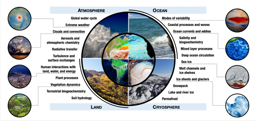
Figure 1:Example of a decomposition of the Earth system based on a domain. [Source]
The first way to decompose the operator is into the core dynamical system that represents processes within the Earth system.
While it is ideal to have all dynamical processes under a single umbrella, it’s more feasible to decompose each into subcomponents. We can do this by decomposing the Earth domain into different sections. There are potentially many ways one can partition the Earth into sections as we can be as granular as possible when describing a dynamical system. However, the Earth is a massive scale and we need to put a limit due to computational constraints.
There are 3 key partitions that are prevalent in the CMIP6 simulations include the atmosphere, the land, and the ocean.
On a high-level, this is a reasonable decomposition. However, depending on your field and beliefs, one could easily decompose this field into other specific dynamical systems that are potentially influential. For example, we could include a vegetation dynamical system and a (sea) ice dynamical system.
In the case of the CMIP6 project, the AMIP6 models only include the atmospheric portion and parameterize the ocean and land (?). However, all other scenarios include each of these dynamical systems within their framework.
Forcings
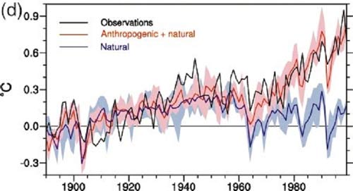
Figure 2:A figure from [Meehl et. al., 2004] showing the anthropogenic plus natural vs. just natural radiative forcing temperature change vs. observed global surface temperature increase. [Source]
We can add another term to our PDE which takes into account any external natural forcings that we think are necessary.
A forcing is essentially an external (or internal) factor that is independent of our defined dynamical system. For example, the wind is a factor of the atmosphere which influences the dynamical system of the ocean system and vice versa.
For the CMIP6 project, we consider 2 broad categories of forcings: natural and anthropogenic.
Natural is anything that we consider is a natural process, e.g., solar radiation, albedo, Milankovitch cycles, natural oscillations, sun spots, and volcanoes. Anthropogenic is anything that we consider is a process or effect that was caused by humans, e.g., greenhouse gases.
One important factor is that forcings come from observations, , when they are available.
The first row showcases the simulations in the historical period where observations are available so these are included within the forcing terms. However, the second row showcases the simulations in the projection period where observations are not available. So the forcing terms are 0.
In the context of the CMIP6 project, they have different forcings available:
- piControl run will include none of the forcings (neither anthropogenic nor natural).
- Historcal-Natural will only include the natural forcing.
- Historical will include both the anthropogenic forcing and the natural forcing.
Note: A key component to note is that these are forcings using observations, and not assimilation.
Below, we have a summary table of the different CMIPX simulations that are available and what distinguishes them.
Table 1:Table of Different CMIP6
| Simulation | Dynamical | Observation Forcing | Anthropogenic Forcing |
|---|---|---|---|
| piControl | Atm, Land, Ocn | No | No |
| Historical-Natural | Atm, Land, Ocn | Yes | No |
| Historical | Atm, Land, Ocn | Yes | Yes |
| GHG | Atm, Land, Ocn | Yes | Yes |
| AMIP5 | Atm, Land | Yes | Yes |
Misc.
There are other important factors to consider when looking at the models.
Ensembles
Many institutions offer a number of different runs, i.e., ensembles.
Scenarios
The strength of the forcing is the focus for the projections. We don’t have observations of the anthropogenic activity, so we need to prescribe this forcing. In general, there are a number of Shared Socioeconomic Pathways (SSP), a.k.a., scenarios provided ranging from optimistic to pessimistic.
SSP Scenarios Summary
Table 2:Table of Different Scenarios
| Scenario Acronym | Label |
|---|---|
| SSP1 | Sustainability |
| Historical-Natural | Atm, Land, Ocn |
| SSP2 | Middle of Road |
| SSP3 | Regional Rivalry |
| SSP4 | Inequality |
| SSP5 | Fossil-Fueled Development |
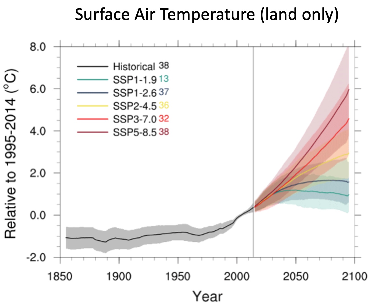
Figure 3:Example of projections with different scenarios for surface air temperature [Source]
Pressure Levels
In the database, there is an option to choose the CMIP6 simulations at pressure levels or at single levels.
Reanalysis
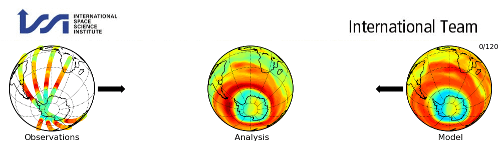
Figure 4:A simple example of data assimilation for an upper atmosphere variable. [Source]
In the above section, we were in the world of simulations which means we were using dynamical models with different forcings. However, an improvement to this would be to incorporate observations of the actual variables we wish to use. This process is usually done through the process of data assimilation (DA). DA is the process of combining observations with physical models.
where is a parameterized transformation that combines the prior state from the dynamical model, , and the observations, .
The main reason why DA is necessary is because the observations almost never exactly match the physical variables we are interested in modeling. For example, they could be sparse/incomplete or they could be completely unobserved. In addition, they could be noisy due to instrument error. For example, we may be interested in the ocean state but we only observe a fraction of the oceans surface [Johnson et al., 2023]. This results in a very high-dimensional system whereby we only have partial observations of a tiny fraction of the system. So it’s absolutely essential to incorporate strong prior information through the form of physical models to try and recover the “true” ocean state.
The ERA5 is the most comprehensive reanalysis dataset available. However, it is worth noting that the ocean component of the ERA5 dataset is really lacklustre compared to the atmospheric and land components. So there are other more comprehensive reanalysis datasets specifically for the oceanic variables, e.g., GLORYS and HYCOM.
List of Datasets
Below is a large list of my datasets.
A quick list of current reanalysis, see this link. They have a comprehensive list of reanalysis available for the atmosphere and the ocean.
Ocean
GLORYS.
A reanalysis dataset for the ocean. It is based on the NEMO model and observations.
It has global coverage with a spatial resolution of 0.083 x 0.083 deg ≈ 9.2 km.
It does have some higher resolution subregions like the Med or Arctic with higher spatial resolutions, e.g., 0.043 x 0.043 deg ≈ 4.8 km.
HYCOM.
A reanalysis dataset for the ocean. It is based on the ... model and observations.
It has global coverage with a spatial resolution of 0.083 x 0.083 deg ≈ 9.2 km.
ORAS5.
A reanalysis dataset for the ocean. It is based on the NEMO model and observations. It has global coverage with a spatial resolution of 0.25 x 0.25 ≈ [25,9] km
Climate
CMIP5 | CMIP6. Some climate projections for the land, atmosphere, and ocean. They feature a historical period from 1850-2014 and a projection period from 2015-2100. The anthropogenic forcing was dictated using different SSP scenarios.
ERA5. This is a reanalysis dataset which are climate models which have assimilated observations.
NCEP. This is a reanalysis dataset from the NOAA/NCAR institutions which for assimilated observations.
- Johnson, J. E., Febvre, Q., Gorbunova, A., Metref, S., Ballarotta, M., Sommer, J. L., & Fablet, R. (2023). OceanBench: The Sea Surface Height Edition. arXiv. 10.48550/ARXIV.2309.15599