Empirical Fit
P-P Plot
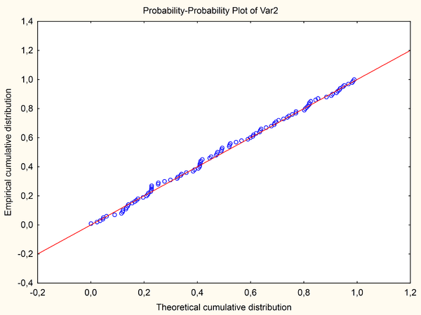
Figure 1:Example of p-p plot from wikipedia. [Source: Wikipedia]
This is also known as the probability-probability plot, the percent-percent plot, or the p-value plot. It is used for assessing how closely two datasets agree and/or the residuals. See wiki for more details.
Note: this plot only works when we have the theoretical cumulative distribution.
Q-Q Plot
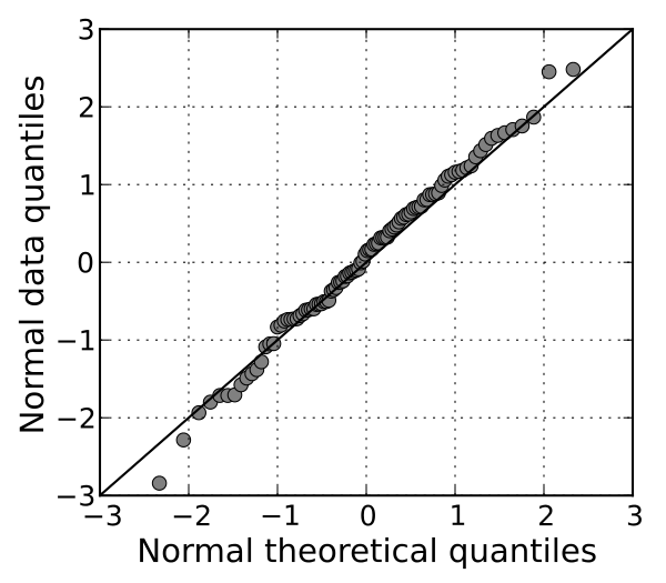
Figure 1:Example of Q-Q plot from wikipedia. [Source: Wikipedia]
This is the quantile-quantile plot. This is a graphical tool to compare two probability distributions by comparing their quantiles versus one another. See wiki for more details.
Predictions
Return Period
We can extrapolate an distribution by computing the -return level (see blog). This represents the high quantile for which the probability that the maximym exceeds this quantile is . This concept is known as the return period. The return period of a particular event is the inverse probability that the event will be exceeded in any given year. For example, the -year return level is associated with a return period of years. The return level is the quantile of an arbitrary quantile function for a distribution.(Mahmoudian & Mahammadzadeh, 2014).
To compute the return level of s.t. the distribution, . We can solve for which results in the following formula.
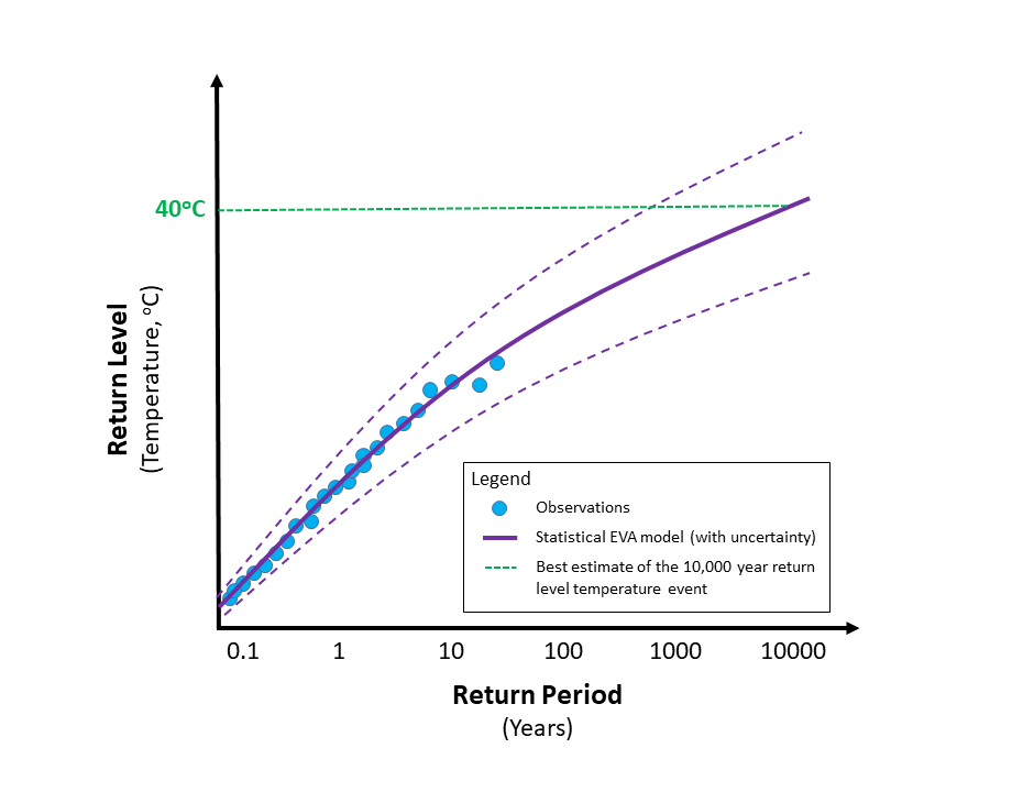
Figure 1:Example of return period for temperature. [Source: MetOffice]
This is also known as the recurrence interval or repeat interval which is an average time or an estimated average time between events. In the case of extreme events, these can include floods, heatwaves, or droughts. See wiki for more details.
Interpretations
Waiting Time - The average waiting time until next occurrence of the event in years.
Number of Events - The average number of events occurring within a -year period.
Example: GEVD
The return period is a nifty tool for making predictions of along the tails of the distribution. We simply need the quantile function for the arbitrary distribution. The quantile function maps some input, , to a threshold value so that the probability of being less than or equal than is .
We can an example for the GEVD. For the GEVD, we have the quantile function defined as
One can easily find this function (along with many others) in a wiki or any similar resource. Now, we simply plug in the return level, i.e., , into the quantile function
Example: GPD
The return period is a nifty tool for making predictions of along the tails of the distribution. We simply need the quantile function for the arbitrary distribution. The quantile function maps some input, , to a threshold value so that the probability of being less than or equal than is .
We can an example for the GEVD. For the GPD, we have to be careful because we don’t have an exact expression.
where is the probability of exceeding the threshold. We can use this to estimate the return level, .
Mean Excess Function
where the scale parameter, , varies linearly in the threshold and the shape parameter ξ is fixed wrt the threshold .
Expected Shortfall
Ultimately, the goal of EVT is to compute the value at risk. We can derive the expected shortfall (conditional rv).
where:
- - the random variable
- μ - the threshold (in percentage terms)
- - number of observations
- - # of observations that exceed the threshold
We can define the expected shortfall (ES) as:
- Mahmoudian, B., & Mohammadzadeh, M. (2014). A spatio-temporal dynamic regression model for extreme wind speeds. Extremes, 17(2), 221–245. 10.1007/s10687-014-0180-2