Problem Category - Research Notebook

Overview¶

Interpolation
Extrapolation, X-Casting
Variable Transformation
Feature Representation
Operator Learning

Interpolation¶

This is when everything is inside the convex hull of a spatial domain and the period of observations. From a spatial perspective, if we can draw a straight-line between the a query point of interest and two other reference points, then I would consider it an interpolation problem.

Examples:

Weather Stations Extremes
SST <--> SSH
MODIS <--> GOES <--> MSG

Extrapolation¶

X-Casting¶

This is the exclusive case when we are trying to predict outside of the period of interest.

HindCasting, $t0 - \tau$
NowCasting, $T + \tau$
ForeCasting, $T+\tau$
Climate Projections, $T+\tau$ ,

Variable Transformation¶

Examples:

SST --> SSH
Satellite Instrument - 2 - Satellite Instrument

Feature Representation¶

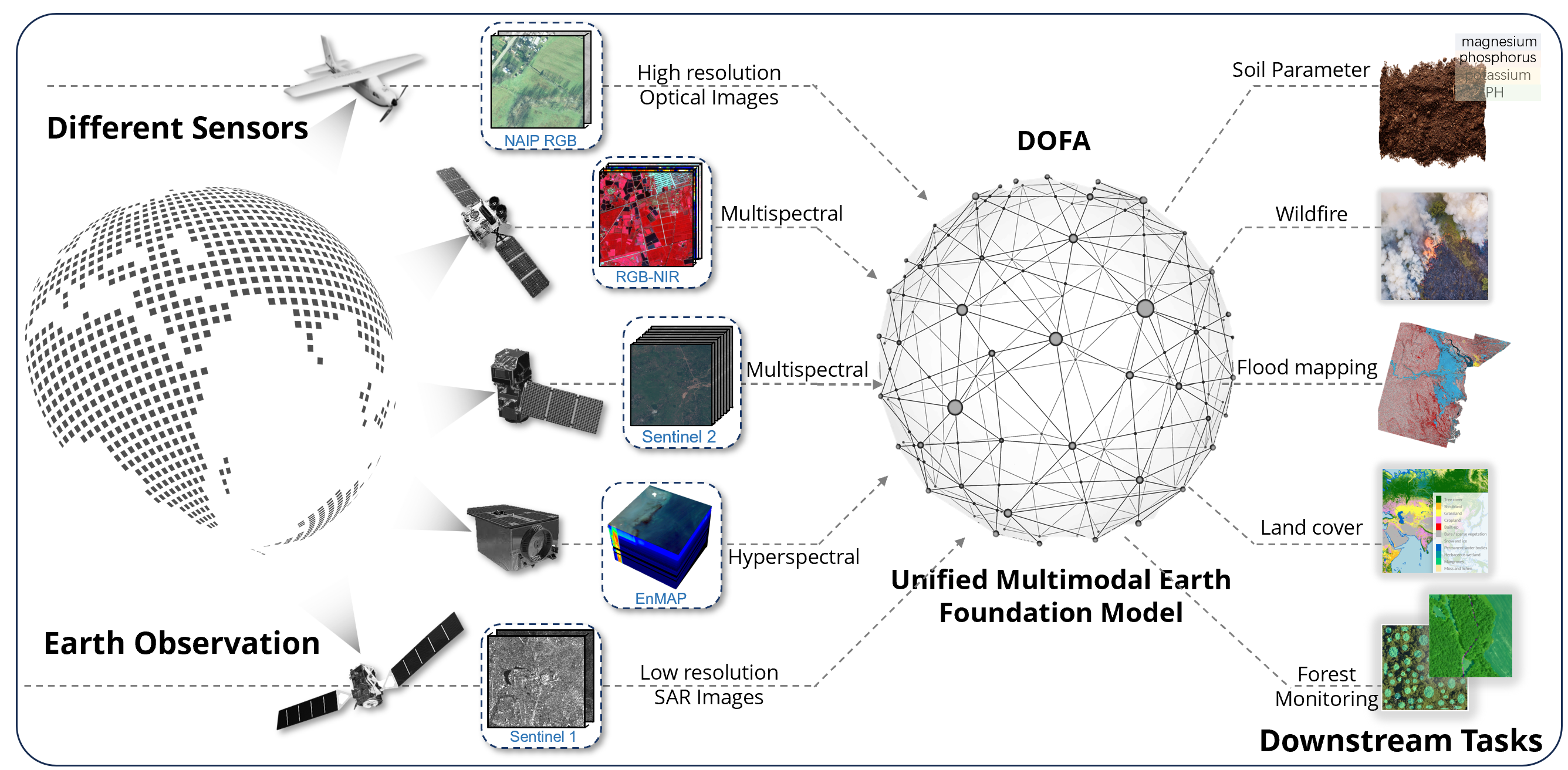
Sunset at the beach — Figure 1:A Model from DOFA whereby they train their model on different modalities for Remote sensing data. Source: GitHub | Paper (arxiv)

This is also known as Representation Learning, Foundational Models

\begin{aligned} \text{Encoder}: && && \mathbf{z} &= \boldsymbol{T}_e\left(\mathbf{y},\boldsymbol{\theta} \right) \\ \text{Decoder}: && && \mathbf{y} &= \boldsymbol{T}_d\left(\mathbf{z},\boldsymbol{\theta} \right) \\ \end{aligned}

(1)

Strategies:

Data Augmentation, e.g., Small-Medium Perturbations
Masking

Examples:

PCA/EOF/POD/SVD
AutoEncoders
Bijective, Surjective, Stochastic
ROM -> AutoEncoders
Linear ROM -> PCA/EOF/POD/SVD, ProbPCA
Simple -> Flow Model
MultiScale -> U-Net

Operator Learning¶

Now, we have broken each of the different problem categories into different subtopics. However, we can easily have a case whereby we have each a single problem category or a combination of all problem categories. There is an umbrella term which encompasses all of the aforementioned stuff.

\begin{aligned} \text{Variable I}: && && \mathcal{X}:\Omega_X\times\mathcal{T}_X\rightarrow\mathcal{X} \\ \text{Variable II}: && && \mathcal{Y}:\Omega_Y\times\mathcal{T}_Y\rightarrow\mathcal{Y} \\ \end{aligned}

(2)

Now, we wish to learn some.

\mathcal{F}: \mathcal{X}\times\mathcal{\Theta} \rightarrow \mathcal{Y}

(3)

Normally, we can break this into steps. This is also known as lift and learn.

\begin{aligned} \text{Encoder}: && && T_e &: \left\{\mathcal{X}:\Omega_X,\mathcal{T}_X \right\} \rightarrow \left\{\mathcal{Z}_X:\Omega_{Z},\mathcal{T}_{Z} \right\} \\ \text{Latent Space Transformation}: && && F_z &: \left\{\mathcal{Z}_X:\Omega_Z,\mathcal{T}_Z \right\} \rightarrow \left\{\mathcal{Z}_Y:\Omega_Z,\mathcal{T}_Z \right\} \\ \text{Decoder}: && && T_d &: \left\{\mathcal{Z}:\Omega_Z,\mathcal{T}_Z \right\} \rightarrow \left\{\mathcal{Y}:\Omega_Y,\mathcal{T}_Y \right\} \end{aligned}

(4)

Learn a good representation network which encodes our data from an infinite domain into a finite latent domain.
Do the computations in finite dimensional space.
Learn a reconstruction function from the finite dimensional latent domain to another infinite dimensional domain.

Examples:

Unstructured <--> Irregular, e.g. CloudSAT + MODIS
Irregular <--> Regular, e.g., AlongTrack + Grid
Regular <--> Regular, e.g., GeoStationary I + GeoStationary II