Gauss-Newton inference for non-conjugate GPs

Gauss-Newton runs the same Newton iteration as Laplace but with a strictly-positive lower bound (a “PSD floor”) on the diagonal site precision:

\Lambda_n = \max\!\left(-\frac{\partial^2 \log p(y_n \mid f_n)}{\partial f_n^2}, \, \tau\right)

((1))

where $\tau > 0$ is the floor. The two strategies differ only in that floor’s default value — Laplace floors at 10^-6, GN floors at 10^-3. Everything else is identical.

Why the floor matters. For log-concave likelihoods (Bernoulli, Poisson) the negative Hessian is positive everywhere, so neither floor bites and GN ≡ Laplace exactly.

For non-log-concave likelihoods — StudentT, mixture-of-Gaussians, anything with heavy tails — the Hessian becomes positive in the tails:

\frac{\partial^2}{\partial f^2} \log p_{\text{StudentT}}(y \mid f, \nu, \sigma) = \frac{(\nu+1)((y-f)^2 - \nu \sigma^2)}{(\nu \sigma^2 + (y-f)^2)^2}

((2))

which is positive whenever $|y-f|^2 > \nu \sigma^2$ (residual “big enough that the heavy tail kicks in”). At those points $-h_n < 0$ . Both Laplace and GN catch this with the floor; GN’s larger floor is just a more conservative safety belt.

What this notebook shows: two regimes of GP-Laplace-style inference. In both, GN and Laplace converge to the same posterior — the floor difference is invisible at convergence. The honest answer to “when do you pick GN over Laplace?” is almost never; pick GN if you want the larger floor as a safety habit, otherwise stick with Laplace. The real cost in non-log-concave problems is the damping parameter, not the floor.

import jax
import jax.numpy as jnp
import matplotlib.pyplot as plt
import numpy as np

from pyrox.gp import (
    RBF,
    BernoulliLikelihood,
    GaussNewtonInference,
    GPPrior,
    LaplaceInference,
    StudentTLikelihood,
)


plt.rcParams["figure.dpi"] = 110
key = jax.random.PRNGKey(0)

/home/azureuser/localfiles/pyrox/.venv/lib/python3.13/site-packages/tqdm/auto.py:21: TqdmWarning: IProgress not found. Please update jupyter and ipywidgets. See https://ipywidgets.readthedocs.io/en/stable/user_install.html
  from .autonotebook import tqdm as notebook_tqdm

Regime 1 — Bernoulli classification (log-concave)¶

Same setup as the Laplace notebook. We expect GN and Laplace to match: the Bernoulli Hessian $-\sigma(f)(1-\sigma(f))$ is always negative, so the floor τ never bites.

N = 60
X = jnp.linspace(-3.0, 3.0, N)[:, None]
f_true = 2.0 * jnp.sin(X[:, 0]) + 0.4 * X[:, 0]
probs_true = jax.nn.sigmoid(f_true)
y_bin = (jax.random.uniform(key, (N,)) < probs_true).astype(jnp.float32)

prior = GPPrior(kernel=RBF(init_lengthscale=0.6, init_variance=1.5), X=X)
lik = BernoulliLikelihood()

cond_lap = LaplaceInference(max_iter=50).fit(prior, lik, y_bin)
cond_gn = GaussNewtonInference(max_iter=50).fit(prior, lik, y_bin)

print(
    f"Laplace        iters={cond_lap.n_iter}  log_marg={float(cond_lap.log_marginal_approx):.4f}"
)
print(
    f"Gauss-Newton   iters={cond_gn.n_iter}  log_marg={float(cond_gn.log_marginal_approx):.4f}"
)
print(
    f"max |q_mean diff|: {float(jnp.max(jnp.abs(cond_lap.q_mean - cond_gn.q_mean))):.2e}"
)
print(
    f"max |q_var diff|:  {float(jnp.max(jnp.abs(cond_lap.q_var - cond_gn.q_var))):.2e}"
)

Laplace        iters=6  log_marg=-25.6915
Gauss-Newton   iters=6  log_marg=-25.6915
max |q_mean diff|: 0.00e+00
max |q_var diff|:  0.00e+00

Identical posteriors to ~ float32 noise. Diagnostic plot of the per-point site precisions confirms the regimes match.

fig, ax = plt.subplots(figsize=(7, 3))
ax.scatter(X[:, 0], np.asarray(cond_lap.site_nat2), s=42, label="Laplace", alpha=0.6)
ax.scatter(X[:, 0], np.asarray(cond_gn.site_nat2), s=14, label="Gauss-Newton")
ax.axhline(
    0.25, color="k", ls="--", lw=0.8, label=r"theoretical max $\sigma(1-\sigma)=1/4$"
)
ax.set_xlabel("x")
ax.set_ylabel(r"$\Lambda_n$")
ax.set_title("Site precision on Bernoulli — Laplace vs GN (identical regime)")
ax.legend(fontsize=8)
plt.tight_layout()
plt.show()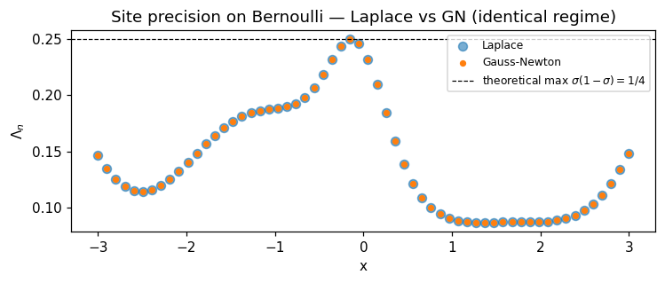

Regime 2 — StudentT regression with outliers (non-log-concave)¶

Here the Hessian goes positive at points where the residual $|y-f|$ is large. Two outliers are planted in an otherwise-clean sinusoid.

key2, key3 = jax.random.split(jax.random.PRNGKey(42), 2)
N = 40
X = jnp.linspace(-3.0, 3.0, N)[:, None]
f_true = jnp.sin(X[:, 0])
y_clean = f_true + 0.1 * jax.random.normal(key2, (N,))
# Plant two outliers
outlier_idx = [12, 28]
y = y_clean.at[outlier_idx[0]].set(4.0).at[outlier_idx[1]].set(-4.0)

prior_t = GPPrior(kernel=RBF(init_lengthscale=0.7, init_variance=1.0), X=X)
lik_t = StudentTLikelihood(df=3.0, scale=0.3)

# Pure Newton oscillates on this non-log-concave likelihood; both strategies
# expose a ``damping`` argument that takes a convex combination of the
# previous iterate and the full Newton step. ``damping=0.3`` converges in
# ~50 iterations.
cond_lap = LaplaceInference(max_iter=200, damping=0.3).fit(prior_t, lik_t, y)
cond_gn = GaussNewtonInference(max_iter=200, damping=0.3).fit(prior_t, lik_t, y)

print(
    f"Laplace         iters={cond_lap.n_iter:3d}  conv={cond_lap.converged}  "
    f"log_marg={float(cond_lap.log_marginal_approx):.3f}"
)
print(
    f"Gauss-Newton    iters={cond_gn.n_iter:3d}  conv={cond_gn.converged}  "
    f"log_marg={float(cond_gn.log_marginal_approx):.3f}"
)

Laplace         iters= 35  conv=True  log_marg=-29.481
Gauss-Newton    iters= 35  conv=True  log_marg=-29.481

Inspect the signed per-point Hessian at convergence — values where $-h_n < 0$ are where Laplace would float its precision down to the floor and GN bumps it up to $\tau = 10^{-3}$ . The outlier points are exactly where the two strategies differ.

def neg_hess_at(f, y, lik):
    def per_n(f_n, y_n):
        return jax.grad(jax.grad(lambda fv: lik.log_prob(fv[None], y_n[None])))(f_n)

    return -jax.vmap(per_n)(f, y)


neg_h_lap = neg_hess_at(cond_lap.q_mean, y, lik_t)
neg_h_gn = neg_hess_at(cond_gn.q_mean, y, lik_t)

fig, axes = plt.subplots(1, 2, figsize=(11, 3.5), sharey=False)
ax = axes[0]
ax.scatter(
    X[:, 0], np.asarray(neg_h_lap), s=20, label=r"raw $-h$ at Laplace mean", color="C0"
)
ax.scatter(
    X[:, 0],
    np.asarray(cond_lap.site_nat2),
    s=18,
    label="Laplace site $\\Lambda_n$",
    facecolors="none",
    edgecolors="C1",
    lw=1.2,
)
ax.axhline(0, color="k", lw=0.5)
for i in outlier_idx:
    ax.axvline(X[i, 0], color="red", alpha=0.25, lw=1)
ax.set_title("Laplace — raw vs floored curvature")
ax.set_xlabel("x")
ax.set_ylabel(r"$-h_n$ / $\Lambda_n$")
ax.legend(fontsize=8)

ax = axes[1]
ax.scatter(
    X[:, 0], np.asarray(neg_h_gn), s=20, label=r"raw $-h$ at GN mean", color="C0"
)
ax.scatter(
    X[:, 0],
    np.asarray(cond_gn.site_nat2),
    s=18,
    label="GN site $\\Lambda_n$",
    facecolors="none",
    edgecolors="C2",
    lw=1.2,
)
ax.axhline(0, color="k", lw=0.5)
ax.axhline(1e-3, color="C2", ls="--", lw=0.8, label=r"GN floor $\tau=10^{-3}$")
for i in outlier_idx:
    ax.axvline(X[i, 0], color="red", alpha=0.25, lw=1)
ax.set_title("Gauss-Newton — raw vs floored curvature")
ax.set_xlabel("x")
ax.legend(fontsize=8)
plt.tight_layout()
plt.show()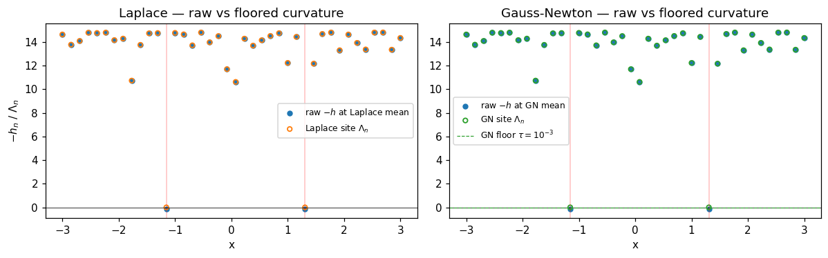

At the two outlier locations, the raw $-h$ goes negative — these points are in the heavy-tail regime, where the StudentT log-likelihood is concave-up (positive curvature), so Newton’s exact-Hessian step would be ill-defined. Both strategies floor the precision at outliers; GN’s larger default floor leaves a more obvious “step up” pattern.

Predictive consequences¶

At convergence the two posteriors are essentially identical — the floor doesn’t bite when both strategies have damped their way to the same fixed point.

X_star = jnp.linspace(-3.5, 3.5, 200)[:, None]
m_lap, v_lap = cond_lap.predict(X_star)
m_gn, v_gn = cond_gn.predict(X_star)
m_lap, v_lap = np.asarray(m_lap), np.asarray(v_lap)
m_gn, v_gn = np.asarray(m_gn), np.asarray(v_gn)
sd_lap = np.sqrt(np.maximum(v_lap, 0))
sd_gn = np.sqrt(np.maximum(v_gn, 0))

fig, axes = plt.subplots(1, 2, figsize=(11, 3.6), sharey=True)
for ax, name, m, sd, color in [
    (axes[0], "Laplace", m_lap, sd_lap, "C0"),
    (axes[1], "Gauss-Newton", m_gn, sd_gn, "C2"),
]:
    ax.fill_between(
        X_star[:, 0], m - 2.0 * sd, m + 2.0 * sd, alpha=0.25, color=color, label="±2σ"
    )
    ax.plot(X_star[:, 0], m, color=color, lw=2, label="posterior mean")
    ax.plot(X[:, 0], jnp.sin(X[:, 0]), "k--", lw=1, label="true f")
    ax.scatter(X[:, 0], y, c="C3", s=14, alpha=0.7)
    ax.scatter(
        X[outlier_idx, 0],
        y[jnp.array(outlier_idx)],
        facecolors="none",
        edgecolors="black",
        s=120,
        lw=1.5,
        label="outliers",
    )
    ax.set_title(name)
    ax.set_xlabel("x")
    ax.set_ylim(-2.0, 2.0)
axes[0].set_ylabel("y / f")
axes[0].legend(fontsize=7, loc="lower left")
fig.suptitle("StudentT regression — Laplace vs GN", y=1.04)
plt.tight_layout()
plt.show()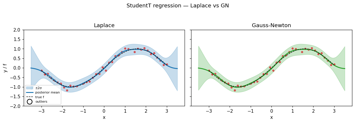

fig, ax = plt.subplots(figsize=(8, 3))
ax.plot(X_star[:, 0], np.abs(m_lap - m_gn), label="|Δ posterior mean|", color="C3")
ax.plot(X_star[:, 0], np.abs(sd_lap - sd_gn), label="|Δ posterior std|", color="C4")
for i in outlier_idx:
    ax.axvline(X[i, 0], color="red", alpha=0.25, lw=1)
ax.set_xlabel("x")
ax.set_ylabel("absolute difference")
ax.set_title("Where Laplace and GN disagree on the StudentT posterior")
ax.legend(fontsize=8)
plt.tight_layout()
plt.show()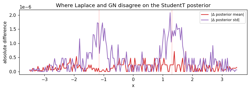

Summary¶

Bernoulli (log-concave): GN ≡ Laplace to numerical precision. The floor is never reached.
StudentT (non-log-concave): the negative Hessian does go negative at outlier locations, but both strategies catch it — Laplace’s 10^-6 floor and GN’s 10^-3 floor both clip those points to a positive precision. The two strategies converge to the same posterior; the difference between the floors only affects intermediate iterates, not the fixed point.
The real lever for non-log-concave problems is damping, not the floor. Pure Newton (damping=1.0) oscillates on StudentT-with-outliers; we set damping=0.3 and both strategies converge in ~35 iterations.

Practical guidance:

On log-concave likelihoods (Bernoulli, Poisson): use Laplace. GN gives the same answer at the same cost.
On non-log-concave likelihoods (StudentT, mixture, etc.): use Laplace with damping ∈ [0.3, 0.7] as the first attempt; switch to GN only if you specifically prefer the more conservative floor for numerical safety. The two strategies will give virtually identical answers when both converge.
The much bigger story in non-log-concave inference is moment matching (EP) and statistical linearization (PL) — they give different posteriors, not just different numerical paths. See those notebooks.

Both strategies share the same API:

cond = prior.condition_nongauss(StudentTLikelihood(df=3, scale=0.3), y,
                                strategy=GaussNewtonInference(damping=0.3))