Posterior Linearization for non-conjugate GPs

Posterior Linearization (PL) is the moment-aware sibling of Laplace. Where Laplace evaluates the gradient and Hessian of $\log p(y \mid f)$ at a single point (the current iterate), PL evaluates them as expectations under the cavity distribution:

\bar g_n = \mathbb{E}_{q^{\setminus n}(f_n)}\!\left[\frac{\partial \log p(y_n \mid f_n)}{\partial f_n}\right], \qquad \bar h_n = \mathbb{E}_{q^{\setminus n}(f_n)}\!\left[\frac{\partial^2 \log p(y_n \mid f_n)}{\partial f_n^2}\right].

((1))

Then a Newton-style site update with these averaged derivatives and the cavity mean $\mu^c_n$ :

\Lambda_n = -\bar h_n, \qquad \lambda_n^{(1)} = \bar g_n + \Lambda_n \,\mu^c_n.

((2))

Where it sits. PL interpolates between Laplace and EP:

Laplace: $g, h$ at the current point. No averaging, fastest, mode-fit.
PL: $\bar g, \bar h$ averaged over the cavity. One quadrature per site per iteration.
EP: full tilted-distribution moments (zeroth, first, second). Two extra integrals per site.

PL is also known under several other names: Iterated Posterior Linearization Filter (IPLF) in state-space tracking, the Bayesian Newton’s Rule (BNR) in variational optimization (Khan & Rue), and Statistical Linear Regression (SLR) updates in Kalman literature. They’re all the same idea: replace point derivatives with expected derivatives.

What this notebook shows. PL’s posterior on Bernoulli falls between Laplace and EP — closer to EP because it captures more of the cavity’s spread than Laplace’s point-derivative does, but not as accurate as full moment matching. Damping behaves similarly to EP.

import jax
import jax.numpy as jnp
import matplotlib.pyplot as plt
import numpy as np

from pyrox.gp import (
    RBF,
    BernoulliLikelihood,
    ExpectationPropagation,
    GPPrior,
    LaplaceInference,
    PosteriorLinearization,
)


plt.rcParams["figure.dpi"] = 110
key = jax.random.PRNGKey(0)

/home/azureuser/localfiles/pyrox/.venv/lib/python3.13/site-packages/tqdm/auto.py:21: TqdmWarning: IProgress not found. Please update jupyter and ipywidgets. See https://ipywidgets.readthedocs.io/en/stable/user_install.html
  from .autonotebook import tqdm as notebook_tqdm

Bernoulli classification — Laplace vs PL vs EP¶

Same dataset as the previous notebooks. Three strategies compared head-to-head.

N = 60
X = jnp.linspace(-3.0, 3.0, N)[:, None]
f_true = 2.0 * jnp.sin(X[:, 0]) + 0.4 * X[:, 0]
probs_true = jax.nn.sigmoid(f_true)
y = (jax.random.uniform(key, (N,)) < probs_true).astype(jnp.float32)

prior = GPPrior(kernel=RBF(init_lengthscale=0.6, init_variance=1.5), X=X)
lik = BernoulliLikelihood()

cond_lap = LaplaceInference(max_iter=50).fit(prior, lik, y)
cond_pl = PosteriorLinearization(max_iter=200, tol=1e-5, damping=0.5).fit(prior, lik, y)
cond_ep = ExpectationPropagation(max_iter=200, tol=1e-5, damping=0.4).fit(prior, lik, y)

print(
    f"Laplace  iters={cond_lap.n_iter:3d}  conv={cond_lap.converged}  log_marg≈{float(cond_lap.log_marginal_approx):.3f}"
)
print(
    f"PL       iters={cond_pl.n_iter:3d}  conv={cond_pl.converged}  log_marg≈{float(cond_pl.log_marginal_approx):.3f}"
)
print(
    f"EP       iters={cond_ep.n_iter:3d}  conv={cond_ep.converged}  log_marg≈{float(cond_ep.log_marginal_approx):.3f}"
)
print()
print("Pairwise differences in posterior (max absolute):")
print(
    f"  |Laplace - PL| mean={float(jnp.max(jnp.abs(cond_lap.q_mean - cond_pl.q_mean))):.3e}  var={float(jnp.max(jnp.abs(cond_lap.q_var - cond_pl.q_var))):.3e}"
)
print(
    f"  |PL      - EP| mean={float(jnp.max(jnp.abs(cond_pl.q_mean - cond_ep.q_mean))):.3e}  var={float(jnp.max(jnp.abs(cond_pl.q_var - cond_ep.q_var))):.3e}"
)
print(
    f"  |Laplace - EP| mean={float(jnp.max(jnp.abs(cond_lap.q_mean - cond_ep.q_mean))):.3e}  var={float(jnp.max(jnp.abs(cond_lap.q_var - cond_ep.q_var))):.3e}"
)

Laplace  iters=  6  conv=True  log_marg≈-25.691
PL       iters= 22  conv=True  log_marg≈-25.752
EP       iters= 27  conv=True  log_marg≈-25.660

Pairwise differences in posterior (max absolute):
  |Laplace - PL| mean=1.735e-01  var=2.136e-02
  |PL      - EP| mean=4.824e-03  var=2.599e-02
  |Laplace - EP| mean=1.691e-01  var=2.202e-02

Reading the numbers: PL sits between Laplace and EP, exactly as theory predicts. The Laplace↔PL difference is comparable to (or smaller than) Laplace↔EP, and the PL↔EP difference is smaller still — they’re computing similar things, just with EP using full tilted moments rather than just expected derivatives.

Decomposing the site update — point vs averaged derivatives¶

To make the difference between Laplace and PL concrete, plot the per-site gradient and Hessian Laplace uses (at the posterior mean) versus what PL averages over the cavity:

def per_point_grad_at(f, y, lik):
    def per_n(f_n, y_n):
        return jax.grad(lambda fv: lik.log_prob(fv[None], y_n[None]))(f_n)

    return jax.vmap(per_n)(f, y)


def per_point_hess_at(f, y, lik):
    def per_n(f_n, y_n):
        return jax.grad(jax.grad(lambda fv: lik.log_prob(fv[None], y_n[None])))(f_n)

    return jax.vmap(per_n)(f, y)


# Laplace: g, h at the posterior mean.
g_lap = per_point_grad_at(cond_lap.q_mean, y, lik)
h_lap = per_point_hess_at(cond_lap.q_mean, y, lik)

# PL: g, h averaged over the cavity at convergence.
cav_prec = jnp.maximum(jnp.reciprocal(cond_pl.q_var) - cond_pl.site_nat2, 1e-6)
cav_var = jnp.reciprocal(cav_prec)
cav_mean = cav_var * (cond_pl.q_mean / cond_pl.q_var - cond_pl.site_nat1)

# Sample-based estimate of E_cav[grad], E_cav[hess] for the plot.
key_eval = jax.random.PRNGKey(7)
n_samples = 4096
eps = jax.random.normal(key_eval, (n_samples, N), dtype=cav_mean.dtype)
samples = cav_mean[None, :] + jnp.sqrt(cav_var)[None, :] * eps

grads_per_sample = jax.vmap(lambda f: per_point_grad_at(f, y, lik))(samples)
hess_per_sample = jax.vmap(lambda f: per_point_hess_at(f, y, lik))(samples)
g_pl = jnp.mean(grads_per_sample, axis=0)
h_pl = jnp.mean(hess_per_sample, axis=0)

fig, axes = plt.subplots(1, 2, figsize=(11, 3.5))
ax = axes[0]
ax.scatter(X[:, 0], np.asarray(g_lap), s=24, label=r"$g_n$ at Laplace mean", color="C0")
ax.scatter(
    X[:, 0],
    np.asarray(g_pl),
    s=14,
    label=r"$\bar g_n = E_{cav}[\partial \log p]$",
    color="C2",
    marker="x",
)
ax.axhline(0, color="k", lw=0.5)
ax.set_xlabel("x")
ax.set_ylabel("per-site gradient")
ax.set_title("Gradient: point (Laplace) vs cavity-averaged (PL)")
ax.legend(fontsize=8)

ax = axes[1]
ax.scatter(
    X[:, 0], np.asarray(-h_lap), s=24, label=r"$-h_n$ at Laplace mean", color="C0"
)
ax.scatter(
    X[:, 0],
    np.asarray(-h_pl),
    s=14,
    label=r"$-\bar h_n = -E_{cav}[\partial^2 \log p]$",
    color="C2",
    marker="x",
)
ax.axhline(0.25, color="k", ls="--", lw=0.6, label=r"max $\sigma(1-\sigma)=1/4$")
ax.set_xlabel("x")
ax.set_ylabel("per-site precision")
ax.set_title("Negative Hessian: point (Laplace) vs cavity-averaged (PL)")
ax.legend(fontsize=8)
plt.tight_layout()
plt.show()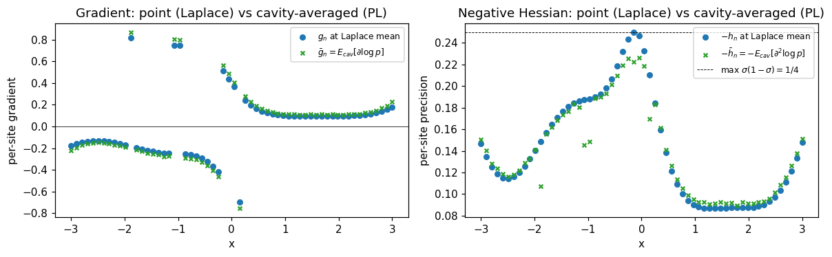

What to notice: averaging over the cavity flattens both the gradient and the negative Hessian relative to the point-evaluation at Laplace’s mode. That’s because the Bernoulli sigmoid saturates — wherever Laplace lands at a point with high curvature, PL’s cavity average pulls in nearby tail values where the sigmoid is flatter. The flatter $\bar h_n$ translates to smaller site precision, which in turn means larger posterior variance under PL than Laplace. Same direction as EP, smaller magnitude.

Predictive comparison¶

X_star = jnp.linspace(-3.5, 3.5, 200)[:, None]
preds = {}
for name, cond in [("Laplace", cond_lap), ("PL", cond_pl), ("EP", cond_ep)]:
    m, v = cond.predict(X_star)
    preds[name] = (np.asarray(m), np.sqrt(np.maximum(np.asarray(v), 0)))

fig, axes = plt.subplots(1, 2, figsize=(11, 3.6), sharey=True)
colors = {"Laplace": "C0", "PL": "C2", "EP": "C3"}

ax = axes[0]
for name, (m, sd) in preds.items():
    ax.fill_between(
        X_star[:, 0], m - 2 * sd, m + 2 * sd, alpha=0.15, color=colors[name]
    )
    ax.plot(X_star[:, 0], m, color=colors[name], lw=2, label=f"{name} mean")
ax.plot(X[:, 0], f_true, "k--", lw=0.8, label="true f")
ax.set_xlabel("x")
ax.set_ylabel("latent f")
ax.set_title("Latent posterior")
ax.legend(fontsize=7, loc="lower right")

ax = axes[1]
for name, (m, sd) in preds.items():
    p_mean = jax.nn.sigmoid(m)
    p_lo = jax.nn.sigmoid(m - 2 * sd)
    p_hi = jax.nn.sigmoid(m + 2 * sd)
    ax.fill_between(X_star[:, 0], p_lo, p_hi, alpha=0.15, color=colors[name])
    ax.plot(X_star[:, 0], p_mean, color=colors[name], lw=2, label=f"{name}")
ax.plot(X[:, 0], probs_true, "k--", lw=0.8, label="true σ(f)")
ax.scatter(X[:, 0], y, c=y, cmap="coolwarm", s=10, alpha=0.6)
ax.set_xlabel("x")
ax.set_ylabel("P(y=1)")
ax.set_title("Predictive probability")
ax.legend(fontsize=7, loc="lower right")
ax.set_ylim(-0.05, 1.05)
plt.tight_layout()
plt.show()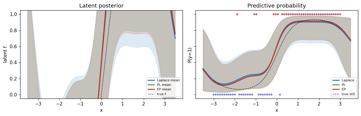

fig, ax = plt.subplots(figsize=(8, 3.5))
m_lap_v, sd_lap_v = preds["Laplace"]
m_pl_v, sd_pl_v = preds["PL"]
m_ep_v, sd_ep_v = preds["EP"]
ax.plot(X_star[:, 0], sd_lap_v, label="Laplace σ", color="C0", lw=2)
ax.plot(X_star[:, 0], sd_pl_v, label="PL σ", color="C2", lw=2)
ax.plot(X_star[:, 0], sd_ep_v, label="EP σ", color="C3", lw=2)
ax.set_xlabel("x")
ax.set_ylabel("posterior std on f")
ax.set_title(
    "Predictive std — Laplace ≤ PL ≤ EP (typical ordering on log-concave likelihoods)"
)
ax.legend(fontsize=8)
plt.tight_layout()
plt.show()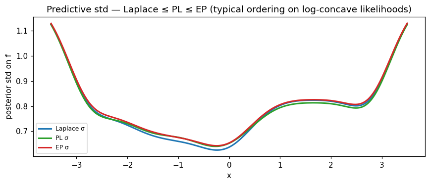

Reading the std panel: the typical ordering on log-concave likelihoods is Laplace ≤ PL ≤ EP — Laplace’s point-Hessian gives the tightest credible intervals (mode-fitting underestimates spread); EP’s full moment matching gives the widest; PL sits between. The differences are biggest in data-sparse regions (here the extrapolation tails) and vanish near densely-observed points where the cavity is tight.

Summary¶

PL = Newton with averaged derivatives. Each site update uses cavity expectations of gradient and Hessian instead of point evaluations.
Sits between Laplace and EP in both philosophy and numerical results: more accurate than Laplace’s mode-fit, less expensive than EP’s full tilted moments. On log-concave likelihoods you get most of EP’s calibration improvement at lower cost per iteration.
Same convergence story as EP. Damping is a speed knob on benign problems, a stability knob on hard ones. Defaults damping=0.5 is reasonable; bump up if convergence is slow, drop if oscillating.
When to pick PL: a sweet-spot for non-Gaussian likelihoods where you want better calibration than Laplace without paying EP’s full cubature cost. Particularly useful for state-space / Markov-GP non-Gaussian inference, where the IPLF formulation is the de facto standard.

cond = prior.condition_nongauss(BernoulliLikelihood(), y,
                                strategy=PosteriorLinearization(damping=0.5))
m, v = cond.predict(X_star)