Learn More

Introduction¶

Definition of Extremes¶

There is no exact definition of an “extreme”. This is because it is an arbitrary classification of a real quantity.

Extreme Indices. These are based on the probability of relative occurrence. For example, we could say that the $90^{th}$ percentile of the observed maximum temperature. We typically assign a threshold which characterizes the severity of a probable outcome should the threshold be crossed. These are typically moderate extremes which are in the $5^{th}$ percentile.

Extreme Value Theory. These are based on a theory called the Extreme Value Theory (EVT). This is a more rigorous definition of extremes which involves more theory. We need EVT because of the sampling issues associated with these rare events; typically we only observe $<1-5\%$ percentile of the total samples. In addition, EVT will allow us to estimate the probability of “values never seen”.

Example¶

For example, if we have a spatiotemporal field of precipitation, we could have different weather regimes. Simply precipitation makes up the bulk of observations, storms could make up the rare events, and hurricanes can make up the extreme events. One could fit a mean regressor on the thunderstorms (given precipitation) and treat the hurricanes as outliers. To estimate the 100-year storm, we would only focus on hurricanes.

Table 1:Extreme Events

Classification	Percentile	Precipitation
Bulk	0.95	Precipitation
Rare Events	0.05	Storms
Extreme Events	0.01	Hurricanes

Formulation¶

Three Interpretations

There are three interpretations of extreme value theory which are complementary. In a nutshell, there are three ways of selecting extreme values from data and then defining a likelihood function.

Max Values —> GEVD
Threshold + Max Values —> GPD
Threshold + Max Values + Counts + Summary Statistic —> PP

Extreme value distributions (EVD) are the limiting distributions for the maximum/minimum of large collections of independent random variables from the same arbitrary distribution.

There are many instances of ways to measure extreme values. In particular, there are 3 ways of defining extremes: 1) maxima, 2) thresholding, 3) counting exceedences. The most common methods are the maxima

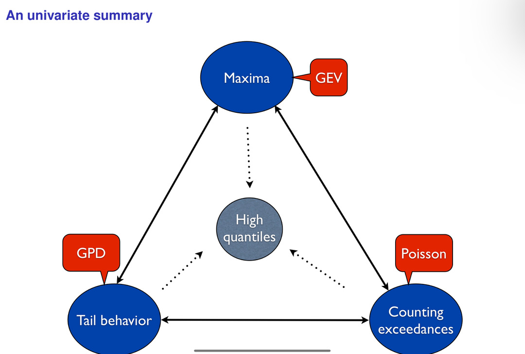
Random image of the beach or ocean! — Figure 1:A figure from Philippe showcasing how we can model extreme values with three different perspectives: 1) maxima values and GEV, 2) tail behaviour with GPD, and 3) counting exceedences with Poisson processes. [Source]

Maxima¶

Here, we are looking at a maximum or minimum within a block of data (see example figure) A block is a set time period such as a week, a month, a season or a year. Note: we have to be careful about what we define as a valid time period because some scales exhibit high variability which could be miscategorized as an extreme. A typical application is to first find the annual maximum value of a spatiotemporal field. We could ask some questions like:

In a given period/patch, how likelihood is an exceedance of a specific threshold?
What threshold can be expected to be exceeded, on average, once every N period/patch?

An advantage of this method is that it is simple to apply and easy to interpret. However, some advantages of this method are that we remove a lot of information which results in framework is not as often directly useful and it is not the most efficient use of a spatiotemporal dataset.

Practical xample: Binning

A very simple example for maximum block estimation is to use a histogram which discretizes a continuous field. We would need to break a continuous field into sufficiently large enough discrete units and take the maximum of each block. A good package is the [`boost-histogram``]() package which works well with spatiotemporal data structures like `xarray`.

First, let’s get some pseudo data

y: Array["Ds Dt"] = ...

Now, we need to describe the spatiotemporal discretization. This can be done via binning.

# create bins
latbins = np.arange(-90, 90, 100)
lonbins = np.arange(-180, 180, 100)
tbins = np.arange("1950", "2020", "Yearly")

Now, we want to take the max value of each bin (TODO)

Generalized Extreme Value Distribution¶

In either case, the Fisher-Tippet Asymptotic Theorem (see wiki | youtube) dictates that extremes generated via a block maxima/minima method will converge to a generalized extreme value distribution (GEVD).

\lim_{n\rightarrow\infty}M_n \sim \text{GEVD}(\mu,\sigma,\xi)

(1)

This basically says that your provided your underlying probability distribution function, $p(\cdot)$ , of a random variable, $y$ , is not highly unsual, regardless of what $p(\cdot)$ is, and provided that the t $n$ is sufficiently large, maxima $\{y\}_+$ samples of size $n$ drawn from $p(\cdot)$ will be distributed as the GEVD.

p(y) \sim \begin{cases} \exp \left[ 1+ \xi \left(\frac{y-\mu}{\sigma}\right)\right]_+^{-1/\xi}, && \xi \neq 0 \\ \exp \left[-\exp\left( - \frac{y - \mu}{\sigma} \right) \right]_+, && \xi=0 \end{cases}

(2)

where $(y)_+=\text{max}\left\{ 0, y \right\}$ , $\boldsymbol{\mu}$ is the location parameter, $\boldsymbol{\sigma}$ is the scale parameter and $\boldsymbol{\xi}$ is the shape parameter. The location parameter, μ, is not the mean of the distribution but rather the center of the distribution. Similarly, the scale parameter, σ, is not the standard deviation of the distribution but rather it governs the size of the deviations about μ. The shape parameter ξ describes the tail behaviour of the GEV distribution which is arguably the most important choice as it dictates the shape of the distribution (see figure). Below, we outline the cases:

Type I. The Gumbel distribution occurs when $\xi=0$ which results in light tails. It is used to model the maximum/minimum of a dataset as it extends over the entire range of real numbers. This is similar to other “light tailed” distributions like the Normal, LogNormal, Hyperbolic, Gamma, and Chi-Squared distributions. This is common when trying to describe the domain of attraction for common distributions like the normal, exponential or gamma. This is not typically found in real world data but there could be some transformed space whereby this is useful.

Type II. The Frechet distribution occurs when $\xi>0$ which results in heavy tails. This is similar to other “heavy tailed” distributions like the InverseGamma, LogGamma, T-student, and Pareto distributions. This is typically found for variables like precipitation / rainfall estimation, stream flow, flood analysis, human lifespan, financial returns and economic damage.

Case III. The Weibull distribution occurs when $\xi<0$ which results in bounded tails. This is similar to the Beta distribution This distribution is common for many variables like temperature, wind speed, pollutants, and sea level. It has also been known to

Once we have the parameters of this distribution, we can calculate the return levels. See my evaluation guide for more information on calculating return levels.

\begin{aligned} \end{aligned}

(3)

Tail Behaviour¶

Often times, we are not interested in the maximum values over a period/block. There are many instances where there is a specific threshold where all values above/below are of interest/concern. In this scenario, we may be interested in using the peaks-over-threshold (PIT) method. The POT approach is based on the idea of modelling data over a high enough threshold. We can select the threshold to trade-off the bias and variance.

F_\mu(y) = \text{Pr}\left\{Y - \mu \leq y|Y>\mu\right\} = \frac{F(y+\mu) - F(\mu)}{1 - F(\mu)}, y > 0

(4)

On one hand, one could select a high threshold which will reduce the number of exceedances. This will increase the estimation variance and the reliability of the parameter estimates. However, this will result in a lower bias because we would get a better approximation of the GPD, i.e., less values --> higher variance, less bias. On the other hand, one could select a lower threshold which will induce a bias because the GPD could fit the exceedances poorly because we have more values, i.e., more values --> less variance, higher bias.

The advantage of this method is that it creates a relevant threshold of interest and it is an efficient use of data because we don’t remove information. The disadvantages of this method is that it is harder to implement and it is difficult to know when the conditions of the theory have been satisfied.

Note: a threshold can be selected by choosing a range of values and seeing which one of them provide a more stable estimation for other parameters. In other words, the estimates for the other parameters should be more or less similar.

Generalized Pareto Distribution¶

According to the Gnedenko-Pickands-Balkema-DeHaan (GPBdH) theorem (see wiki | youtube), using the POT method will converge to the generalized Pareto distribution (GPD) (Gilleland & Katz, 2016), i.e.

\lim_{u\rightarrow\infty} F_u(y) \sim \text{GPD}(\mu, \sigma,\xi)

(5)

This basically says that your provided your underlying probability distribution function, $p(\cdot)$ , of a random variable, $y$ , is not highly unsual, regardless of what $p(\cdot)$ is, and provided that the threshold $u$ is sufficiently large, exceedances of $u$ will be distributed as the Generalized Pareto Distribution (GPD).

p(y) \sim \begin{cases} 1 - \left[ 1 + \xi \left( \frac{y - u}{\sigma_u} \right)\right]_+^{-1/xi}, && \xi \neq 0 \\ 1 - \left[ \exp\left(- \frac{y - u}{ \sigma_u}\right)\right]_+, && \xi=0 \end{cases}

(6)

where $u$ is the high threshold st $y>u$ , $\sigma_u>0$ is the scale parameter which depends on the threshold of $u$ , and $0<\xi<0$ is a the shape parameter. Similar to the GEVD, the shape parameter, ξ, determines the shape of the distribution and it is often very hard to fit. We outline some staple types of distributions defined by the shape parameter below.

Case I. The Pareto distribution occurs when $\xi>0$ which results in heavy tails. This is similar to “heavy-tailed” distributions like the Pareto-type distributions.

Case II. The expontial distribution occurs when $\xi\rightarrow 0$ which results in light tails. This is similar to other “light tail” distributions like the exponential-type distribution.

Case III. The Beta distribution occurs when $\xi<0$ which results in bounded tails. This is similar to other “bounded tailed” distributions like the Beta-type distributions.

Counting Exceedences (TODO)¶

We can use a counting process to model extremes: we count the excesses, i.e., the extreme values, $y$ , that fall above/below a threshold, ε.

Poisson Process (TODO)¶

This would be modelled as a sum of random binary events where the variable $N_n$ counds the number of variables about the threshold, $\epsilon_n$ which has a mean $n$ of $Pr(Y > \epsilon_n)$ . Poisson’s theorem shows us that if $\epsilon_n$ st

\lim_{n\rightarrow\infty} n Pr(Y > \epsilon_n) = \lambda \in (0, \infty)

(7)

then $N_n$ follows approximately a Poisson variable $N$ . This is analogous to counting maximum/minimum values, i.e.,

Pr(M_n \leq \epsilon_n) = Pr(N_n=0)

(8)

where $M_n = \text{max}(Y_1, Y_2, \ldots, Y_n)$ . Poisson’s work shows

\begin{aligned} \lim_{n\rightarrow\infty}Pr(M_n\leq\epsilon_n) &= \lim_{n\rightarrow\infty}Pr(N_n=0)\\ &= Pr(N=0) \\ &=\exp(-\lambda) \end{aligned}

(9)

p\{N>0\} = 1 - \exp(-n\lambda)

(10)

Max-Stable Process¶

Let $\{\boldsymbol{y}(\mathbf{x},t)\}$ be a stochastic process with continuous sample paths. We assume that we have $N$ IID copies of $\boldsymbol{y}$ available. We denote these samples by $\boldsymbol{y}_n$ where $n=1,2,\ldots,N$ and $N\in\mathbb{N}$ denotes the independent replications/realizations.

Let $\{ \boldsymbol{M}_n[\boldsymbol{y}](\mathbf{x},t) \}$ be the pointwise maximum of the underlying process $\boldsymbol{y}_n$ . We can write this explicitly as

\begin{aligned} \boldsymbol{M}[\boldsymbol{y}](\mathbf{x},t) := \text{max}_{n=1,2,\ldots,N} \hspace{2mm} \boldsymbol{y}_n(\mathbf{x},t) && && \forall \hspace{2mm} \mathbf{x}\in\mathcal{X}, && t\in\mathcal{T} \end{aligned}

(11)

Our interest is only in the limiting process of $\boldsymbol{M}_n[\boldsymbol{y}](\mathbf{x},t)$ for $n\rightarrow \infty$ because it may provide an appropriate model in order to describe the behaviour of extremes. In particular, EVT says that if there exists a continuous function

\begin{aligned} \boldsymbol{z}(\mathbf{x},t) &= \lim_{n\rightarrow\infty} \left\{ \frac{\boldsymbol{M}_n(\mathbf{x},t) - \boldsymbol{b}_n(\mathbf{x},t)}{\boldsymbol{a}_n(\mathbf{x},t)}\right\} \\ \boldsymbol{a}_n &= \boldsymbol{a}_n(\mathbf{x},t), && && \boldsymbol{a}_n:\mathbb{R}^{D_s}\times\mathbb{R}^+\rightarrow \mathbb{R}^{D_y} \\ \boldsymbol{b}_n &= \boldsymbol{b}_n(\mathbf{x},t), && && \boldsymbol{b}_n:\mathbb{R}^{D_s}\times\mathbb{R}^+\rightarrow \mathbb{R}^{D_y} \end{aligned}

(12)

and it has a non-degenerate marginal distribution $\forall \mathbf{x}\in\mathcal{X}$ , then this defines an extreme-value process.

Problems

Spatiotemporal Dependencies - representation
Measurements - very little, rare/extremely rare # of observations and complex
Modeling - difficult with little measurements, even with simulations, things are complex and heavy, lose interpretability
Experiment - what’s counterfactual?
Causality - event attribution and direction

Resources¶

Presentation by Reider (2014) - Slides (PDF)
Extreme Value Theory: A Practical Introduction - Herman (200..) - Slides (PDF)

References¶

Gilleland, E., & Katz, R. W. (2016). extRemes2.0: An Extreme Value Analysis Package inR. Journal of Statistical Software, 72(8). 10.18637/jss.v072.i08

Basics

Feature Extraction