Tutorial — Build a bigger graph
Builds an anomaly detector for a stack of multi-channel images as one
Graph: satellite scenes, microscope fields or telescope exposures read
the same way. Six small domain operators do the science; pipekit's own
operators do the plumbing (parallel reads, retries, a cache, shape
checks, a branch, a second input, an observer and a summary).
Time: ~15 minutes.
Prerequisites:
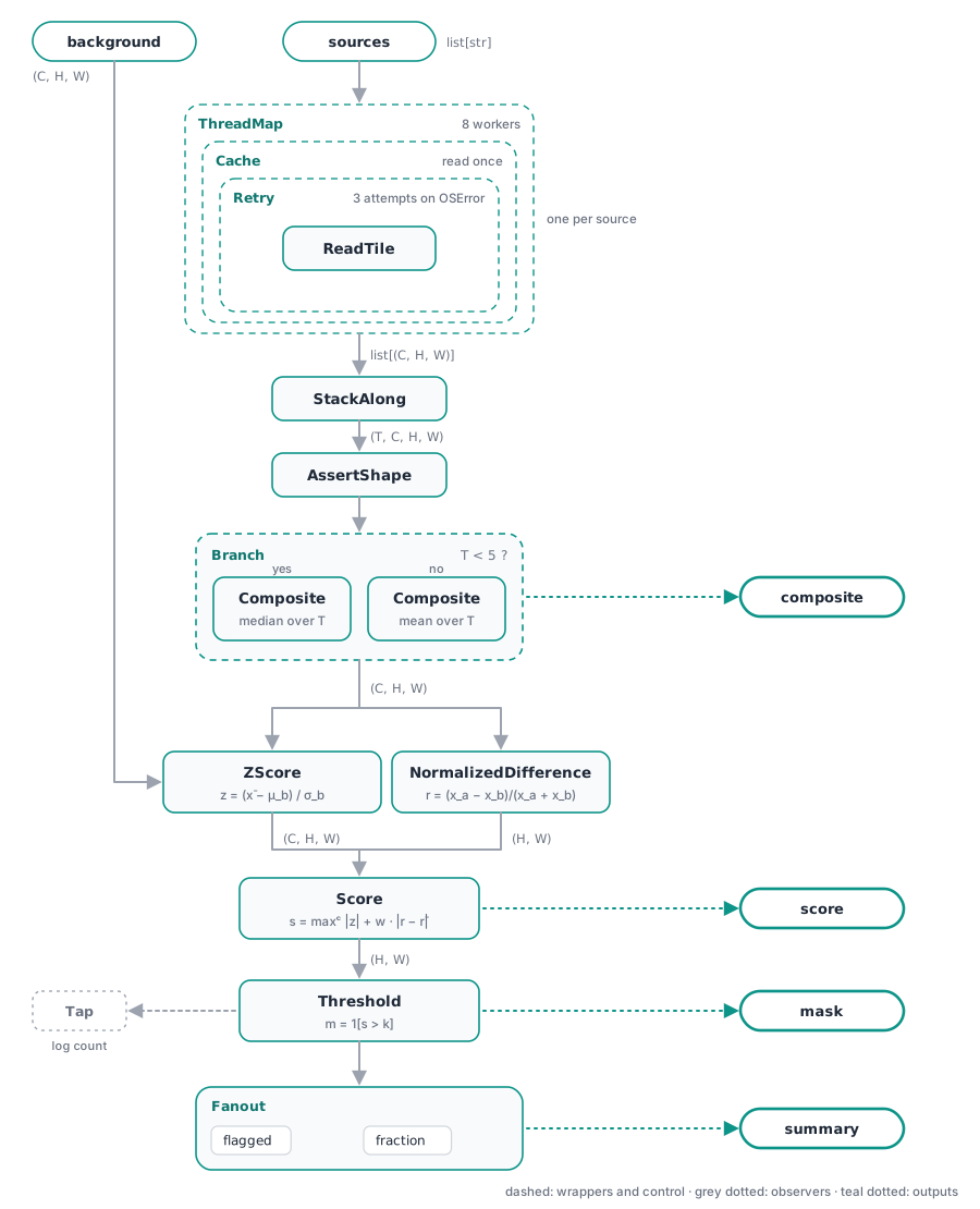
Every box in the figure is one line of code below. The code blocks run in order as one script.
Step 1 — The domain operators
The shapes are declared once, as jaxtyping aliases, and every _apply
below is annotated with them.
from __future__ import annotations

from typing import Any

import numpy as np
from jaxtyping import Bool, Float
from pipekit import (
    AssertShape,
    Branch,
    Cache,
    Fanout,
    Graph,
    Input,
    Operator,
    Retry,
    Sequential,
    Tap,
    ThreadMap,
)
from pipekit_array import StackAlong


# ── shapes ───────────────────────────────────────────────────────────────────
# T  exposures in the stack (6 in the example)
# C  channels (3)
# H  image rows (64)
# W  image columns (64)
Stack = Float[np.ndarray, "T C H W"]
Image = Float[np.ndarray, "C H W"]
Map = Float[np.ndarray, "H W"]
Mask = Bool[np.ndarray, "H W"]

C: int = 3
H: int = 64
W: int = 64
These six classes are the science. Each takes its configuration as
keyword-only constructor arguments and does one thing in _apply.
ReadTile is a stand-in for your reader: it synthesises a noisy
exposure with a small bright patch in channel 0, so the detector has
something to find.
class ReadTile(Operator):
    """Source id ↦ one exposure x ∈ ℝ^{C×H×W}; a stand-in for your reader."""

    def _apply(self, source: str) -> Image:
        # seed = ∑ ord(character): one fixed seed per source id
        seed = 0
        for character in source:
            seed += ord(character)
        rng = np.random.default_rng(seed)
        # x_{chw} = 100 + ε_{chw},  ε ~ 𝒩(0, 1)
        x = 100.0 + rng.normal(0.0, 1.0, (C, H, W))
        # a bright 6 × 6 patch in channel 0: something real, in every exposure
        x[0, 20:26, 30:36] += 8.0
        return x


class Composite(Operator):
    """X ∈ ℝ^{T×C×H×W} ↦ x̄ ∈ ℝ^{C×H×W}, by median or mean over the stack."""

    def __init__(self, *, how: str) -> None:
        self.how = how

    def _apply(self, stack: Stack) -> Image:
        # x̄_{chw} = median_t X_{tchw}
        if self.how == "median":
            return np.median(stack, axis=0)
        # x̄_{chw} = (1/T) ∑_t X_{tchw}
        return np.mean(stack, axis=0)


class ZScore(Operator):
    """z = (x̄ − μ_b) / σ_b, against a background μ_b and its spread σ_b."""

    def __init__(self, *, sigma: float) -> None:
        self.sigma = sigma

    def _apply(self, composite: Image, background: Image) -> Image:
        # z_{chw} = (x̄_{chw} − μ_{b,chw}) / σ_b
        return (composite - background) / self.sigma


class NormalizedDifference(Operator):
    """r = (x_a − x_b) / (x_a + x_b), a ratio between channels a and b."""

    def __init__(self, *, a: int, b: int) -> None:
        self.a = a
        self.b = b

    def _apply(self, x: Image) -> Map:
        xa = x[self.a]
        xb = x[self.b]
        # r_{hw} = (x_{a,hw} − x_{b,hw}) / (x_{a,hw} + x_{b,hw})
        return (xa - xb) / (xa + xb)


class Score(Operator):
    """s = max_c |z_c| + w · |r − r̄|: how unusual each pixel is."""

    def __init__(self, *, weight: float) -> None:
        self.weight = weight

    def _apply(self, z: Image, ratio: Map) -> Map:
        # max_c |z_{chw}|: the most unusual channel per pixel
        worst_channel = np.abs(z).max(axis=0)
        # |r_{hw} − r̄|, r̄ = mean of r over all pixels
        ratio_departure = np.abs(ratio - ratio.mean())
        # s_{hw} = max_c |z_{chw}| + w · |r_{hw} − r̄|
        return worst_channel + self.weight * ratio_departure


class Threshold(Operator):
    """m = 1[s > k]: the anomaly mask."""

    def __init__(self, *, k: float) -> None:
        self.k = k

    def _apply(self, score: Map) -> Mask:
        # m_{hw} = 1[s_{hw} > k]
        return score > self.k
Step 2 — Read in parallel, safely
Reading is where real pipelines fail: a flaky disk or network, the same
file asked for twice. Wrappers take an operator and return one, so they
nest: Retry re-runs a failed read, Cache keeps each source's result
so it is read once, and ThreadMap maps the whole thing over the list
of sources on eight threads. StackAlong (from pipekit-array) stacks
the exposures, and AssertShape fails early if a reader returned the
wrong shape.
Each step is one named variable; | bundles them into load, which
then runs once on the example inputs. Steps 3–5 follow the same
pattern, and Step 6 wires the same steps into a graph.
# the example inputs

# T = 6 source ids
source_ids: list[str] = [f"scene-{i:02d}" for i in range(6)]
# μ_b = 100 in every channel and pixel
flat_background: Image = np.full((C, H, W), 100.0)

# the steps

# source id ↦ x ∈ ℝ^{C×H×W}
read_tile = ReadTile()
# on OSError, read again: up to 3 attempts, backing off from 0.5 s
retried_read = Retry(read_tile, attempts=3, base_delay=0.5, on=(OSError,))
# keep each source's exposure, so no source is read twice
cached_read = Cache(retried_read)
# [s_1, …, s_T] ↦ [x_1, …, x_T], on 8 threads
read = ThreadMap(cached_read, n_workers=8)
# [x_1, …, x_T] ↦ X ∈ ℝ^{T×C×H×W}
stack_exposures = StackAlong(axis=0)
# fail early unless X has shape (T, C, H, W), for any T
check_shape = AssertShape((None, C, H, W))

# the bundle

load: Sequential = read | stack_exposures | check_shape

# run it once, on the example sources

# six exposures, stacked and checked
stack: Stack = load(source_ids)
Step 3 — Choose the composite
Branch routes on a predicate of its input, here the named function
few_exposures. With few exposures the median resists an outlier; with
many the mean is cheaper and as good.
def few_exposures(stack: Stack) -> bool:
    """True when the stack is short enough that the median is worth its cost."""
    # T < 5
    return stack.shape[0] < 5


# the steps

# x̄ = median_t X: resists an outlier among few exposures
median_composite = Composite(how="median")
# x̄ = (1/T) ∑_t X: cheaper, and as good with many
mean_composite = Composite(how="mean")
# x̄ = median_t X when T < 5, else mean_t X
choose_composite = Branch(
    few_exposures,
    if_true=median_composite,
    if_false=mean_composite,
)

# run it once

# T = 6, so the mean
composite: Image = choose_composite(stack)
Step 4 — Join a second input and score
An operator with two arguments joins two branches of the graph. Here
ZScore takes the composite and the background input; the channel
ratio branches off the same composite, and Score joins the two again.
# the steps

# z = (x̄ − μ_b) / σ_b,  σ_b = 1
z_score = ZScore(sigma=1.0)
# r = (x̄_0 − x̄_1) / (x̄_0 + x̄_1): channel 0 against channel 1
channel_ratio = NormalizedDifference(a=0, b=1)
# s = max_c |z_c| + w · |r − r̄|,  w = 10
score_pixels = Score(weight=10.0)

# run it once

# the composite joined with the background
z: Image = z_score(composite, flat_background)
# a branch off the same composite
ratio: Map = channel_ratio(composite)
# the two branches joined again
score: Map = score_pixels(z, ratio)
Step 5 — Observe and summarise
Tap runs a side effect (here, the log line log_flagged) and passes
its input on unchanged. Fanout runs several operators on the same
input and returns a dict of their results; here two small operators,
CountFlagged and FlaggedFraction.
def log_flagged(mask: Mask) -> None:
    """Print how many pixels the mask flags."""
    print(f"{int(mask.sum())} pixels flagged")


class CountFlagged(Operator):
    """n = ∑_{hw} m_{hw}: the number of flagged pixels."""

    def _apply(self, mask: Mask) -> int:
        # n = ∑_{hw} m_{hw}
        return int(mask.sum())


class FlaggedFraction(Operator):
    """f = n / (H · W): the fraction of pixels flagged."""

    def _apply(self, mask: Mask) -> float:
        # f = (1 / (H · W)) ∑_{hw} m_{hw}
        return float(mask.mean())


# the steps

# m = 1[s > k],  k = 3
threshold = Threshold(k=3.0)
# print n, pass m on unchanged
report = Tap(log_flagged)
# n = ∑_{hw} m_{hw}
count_flagged = CountFlagged()
# f = n / (H · W)
flagged_fraction = FlaggedFraction()
# m ↦ {"flagged": n, "fraction": f}
summarise = Fanout({"flagged": count_flagged, "fraction": flagged_fraction})

# the bundle

flag: Sequential = threshold | report

# run it once

# prints "36 pixels flagged"
mask: Mask = flag(score)
# {"flagged": 36, "fraction": 0.0087890625}
summary: dict[str, int | float] = summarise(mask)
Step 6 — Wrap it in a Graph and run it
A graph starts from named Inputs. Calling an operator on an Input
(or on the result of another call) records a node instead of running,
so the named steps of steps 2–5, called on nodes, record the detector
once.
Graph names the inputs and the outputs; everything between them is
what those calls recorded. Run it with keyword arguments, one per
input; it returns a dict, one entry per output.
# wired as a graph: the same steps, called on nodes instead of values

sources_in = Input("sources")
background_in = Input("background")
stack_node = load(sources_in)
composite_node = choose_composite(stack_node)
z_node = z_score(composite_node, background_in)
ratio_node = channel_ratio(composite_node)
score_node = score_pixels(z_node, ratio_node)
mask_node = flag(score_node)
summary_node = summarise(mask_node)

detector = Graph(
    inputs={"sources": sources_in, "background": background_in},
    outputs={
        "composite": composite_node,
        "score": score_node,
        "mask": mask_node,
        "summary": summary_node,
    },
)

# run it: one keyword per input, one entry per output

out: dict[str, Any] = detector(sources=source_ids, background=flat_background)
# the shape of each array output, and the summary as it is
print({k: getattr(v, "shape", v) for k, v in out.items()})
36 pixels flagged
36 pixels flagged
{'composite': (3, 64, 64), 'score': (64, 64), 'mask': (64, 64), 'summary': {'flagged': 36, 'fraction': 0.0087890625}}
The 36 flagged pixels are the 6 × 6 patch ReadTile put in channel 0.
The Tap fires on every run: once for the eager run in Step 5, once for
the graph.
Make it yours
- Another science, another reader. Replace
ReadTilewith whatever returns your carrier: a FITS cube, a microscope field, a satellite scene through geotoolz. Nothing downstream changes as long as the shape does;AssertShapetells you when it does not. - Change a setting, not the code. Every operator keeps its
configuration (
Threshold(k=3.0),Composite(how="median")), so a different threshold or composite is a constructor argument. - Save an operator's configuration.
pipekit.dumps(op)writes any operator's configuration as JSON;pipekit.loadsrebuilds single operators (nested ones need a YAML or Hydra loader).
Where next
- Concepts: the model behind
Operator,SequentialandGraph. - Run a DA cycle: the same interface stepping through time.
- Train an emulator: an operator that learns.