Missing Mass Paradox — Monte Carlo proof

The missing mass paradox¶

A satellite alerting system simultaneously overestimates the average emission rate of a facility while strictly underestimating the total emitted mass. This is the missing mass paradox, and it is a direct consequence of running a size-dependent detection filter over a heavy-tailed mark distribution. This notebook demonstrates the paradox numerically using the plumax.population.paradox library.

The architecture has three strictly separated layers:

Event generator — homogeneous Poisson process generates $N_{\text{true}} \sim \text{Poisson}(\Lambda_{\text{true}})$ events on a timeline, with $\Lambda_{\text{true}} = \lambda_{\text{true}} \cdot T$ .
Mark generator — each event is assigned a flux rate $Q_i \sim \text{LogNormal}(\mu, \sigma)$ [kg/hr]. Heavy-tailed: a few catastrophic blowouts dominate the total mass budget.
Atmospheric filter — each event is thinned independently with Bernoulli probability $P_d(Q_i) = \sigma(k(Q_i - Q_{50}))$ . Small leaks are invisible; large leaks are always detected.

The two proofs we will verify by Monte Carlo are:

\text{PROOF 1:}\quad \mathbb{E}[Q_{\text{obs}}] > \mathbb{E}[Q_{\text{true}}] \qquad\text{(average overestimation)}

(1)

\text{PROOF 2:}\quad M_{\text{obs}} < M_{\text{true}} \qquad\text{(mass underestimation)}

(2)

import warnings


warnings.filterwarnings("ignore", message=r".*IProgress.*")

import dataclasses

import matplotlib.pyplot as plt
import numpy as np
from IPython.display import Markdown

from plumax.population import (
    FacilityConfig,
    build_canonical_scenarios,
    compute_E_Pd,
    logistic_pod,
    lognormal_pdf,
    simulate_paradox,
)


rng_global = np.random.default_rng(0)

1. A single canonical scenario (realistic multi-satellite constellation)¶

We pick an “Active Compressor” setup with a detection midpoint $Q_{50}=1000$ kg/hr and a gradual sigmoid $k=0.003$ . That threshold is chosen to be representative of the mixed sparse-revisit constellation actually in orbit today — Sentinel-2, Landsat-8/9, EMIT, EnMAP, PRISMA, TROPOMI, Sentinel-3 — where the least-sensitive platform in a given overpass sets the effective floor. Hyperspectral hyperspecifics like GHGSat/Tanager are an order of magnitude more sensitive, but any stacked “any-satellite” PoD is dragged up by the multispectral majority.

Consequence: the satellite sees a small fraction of the true events, and the observed sample is heavily biased toward super-emitters. That is exactly what we want to visualise.

cfg = FacilityConfig(
    name="Active Compressor (S2/L8/EMIT/EnMAP/PRISMA/TROPOMI mix)",
    lambda_true=3.0,
    mu=3.0,
    sigma=1.2,
    Q_50=1000.0,
    k=0.003,
    duration=2.0,
    observation_window=365.0,
    seed=123,
)

result = simulate_paradox(cfg)

Markdown(
    "| quantity | value | units |\n"
    "|---|---:|---|\n"
    f"| $N_{{\\text{{true}}}}$ (Poisson draw) | {result.N_true:,d} | events |\n"
    f"| $N_{{\\text{{obs}}}}$ (after POD thinning) | {result.N_obs:,d} | events |\n"
    f"| surviving fraction | {result.N_obs / result.N_true:.3%} | — |\n"
    f"| $\\mathbb{{E}}[P_d]$ (quadrature) | {result.E_Pd:.4f} | — |\n"
    "| | | |\n"
    f"| $\\mathbb{{E}}[Q_{{\\text{{true}}}}]$ (MC) | {result.E_Q_true_mc:,.1f} | kg hr⁻¹ |\n"
    f"| $\\mathbb{{E}}[Q_{{\\text{{obs}}}}]$ (MC) | {result.E_Q_obs_mc:,.1f} | kg hr⁻¹ |\n"
    f"| **average overestimation** $\\mathbb{{E}}[Q_{{\\text{{obs}}}}]/\\mathbb{{E}}[Q_{{\\text{{true}}}}]$ (> 1 ⇒ PROOF 1) | **{result.average_overestimation_ratio:.3f}** | — |\n"
    "| | | |\n"
    f"| $M_{{\\text{{true}}}}$ (MC) | {result.M_true_mc:,.0f} | kg |\n"
    f"| $M_{{\\text{{obs}}}}$ (MC) | {result.M_obs_mc:,.0f} | kg |\n"
    f"| **mass underestimation** $M_{{\\text{{obs}}}}/M_{{\\text{{true}}}}$ (< 1 ⇒ PROOF 2) | **{result.mass_underestimation_ratio:.3f}** | — |\n"
    f"| **MMSF** = $M_{{\\text{{true}}}}/M_{{\\text{{obs}}}}$ | **{result.MMSF:.2f}** | — |\n"
)

The ratios confirm both proofs on a single Monte Carlo realisation. The average observed emission rate is inflated above the true average, while the total observed mass is a fraction of the true mass. The Missing Mass Scaling Factor (MMSF = $M_{\text{true}}/M_{\text{obs}}$ ) quantifies how much the satellite is underreporting in a single number.

2. The three-phase visual proof¶

Three plots tell the full story: timeline thinning (what events survived), distribution warping (how the flux histogram gets biased), and the PoD filter overlay (which events the filter kills).

fig, axes = plt.subplots(1, 3, figsize=(16, 4.5))

ax_timeline, ax_pdf, ax_pod = axes

# --- Phase 1: Timeline Thinning ---
rng_viz = np.random.default_rng(cfg.seed + 9999)
t_true = np.sort(rng_viz.uniform(0, cfg.observation_window, size=result.N_true))
pod_vals = logistic_pod(result.marks_true, cfg.Q_50, cfg.k)
survived = rng_viz.uniform(size=result.N_true) < pod_vals

ax_timeline.eventplot(
    [t_true, t_true[survived]],
    colors=["#888", "#c0392b"],
    linelengths=0.7,
    lineoffsets=[1, 0],
)
ax_timeline.set_yticks([0, 1])
ax_timeline.set_yticklabels(["Observed", "True"])
ax_timeline.set_xlabel("Time (days)")
ax_timeline.set_title(f"Timeline thinning: {result.N_obs}/{result.N_true} survived")

# --- Phase 2: Distribution Warping ---
q_grid = np.logspace(-1, 5, 500)
f_true = lognormal_pdf(q_grid, cfg.mu, cfg.sigma)
pod_grid = logistic_pod(q_grid, cfg.Q_50, cfg.k)
f_obs_unnorm = f_true * pod_grid
norm_const = np.trapezoid(f_obs_unnorm, q_grid)
f_obs = f_obs_unnorm / norm_const if norm_const > 0 else f_obs_unnorm

ax_pdf.semilogx(q_grid, f_true, "k-", lw=2, label="$f(Q)$ true")
ax_pdf.semilogx(
    q_grid, f_obs, "#c0392b", lw=2, label="$f_{\\rm obs}(Q)$ satellite-weighted"
)
ax_pdf.axvline(cfg.Q_50, color="#2c3e50", ls=":", label=f"$Q_{{50}}={cfg.Q_50}$")
ax_pdf.axvline(
    result.E_Q_true_mc, color="k", ls="--", alpha=0.6, label="$E[Q_{\\rm true}]$"
)
ax_pdf.axvline(
    result.E_Q_obs_mc, color="#c0392b", ls="--", alpha=0.8, label="$E[Q_{\\rm obs}]$"
)
ax_pdf.set_xlabel("Q (kg/hr)")
ax_pdf.set_ylabel("density")
ax_pdf.set_title("Distribution warping")
ax_pdf.legend(loc="upper right", fontsize=8)

# --- Phase 3: PoD overlay ---
ax_pod.semilogx(q_grid, pod_grid, "#2c3e50", lw=2, label="$P_d(Q)$")
ax_pod.axvline(cfg.Q_50, color="#2c3e50", ls=":", alpha=0.5)
ax_pod.axhline(0.5, color="#2c3e50", ls=":", alpha=0.5)
ax_pod.fill_between(
    q_grid,
    0,
    pod_grid * f_true / f_true.max(),
    alpha=0.25,
    color="#c0392b",
    label="detected mass density",
)
ax_pod.set_xlabel("Q (kg/hr)")
ax_pod.set_ylabel("$P_d$")
ax_pod.set_ylim(0, 1.05)
ax_pod.set_title(f"Filter strength: E[$P_d$] = {result.E_Pd:.3f}")
ax_pod.legend(loc="center right", fontsize=8)

fig.suptitle(f"Missing Mass Paradox — {cfg.name}", fontsize=12, y=1.02)
fig.tight_layout()
plt.show()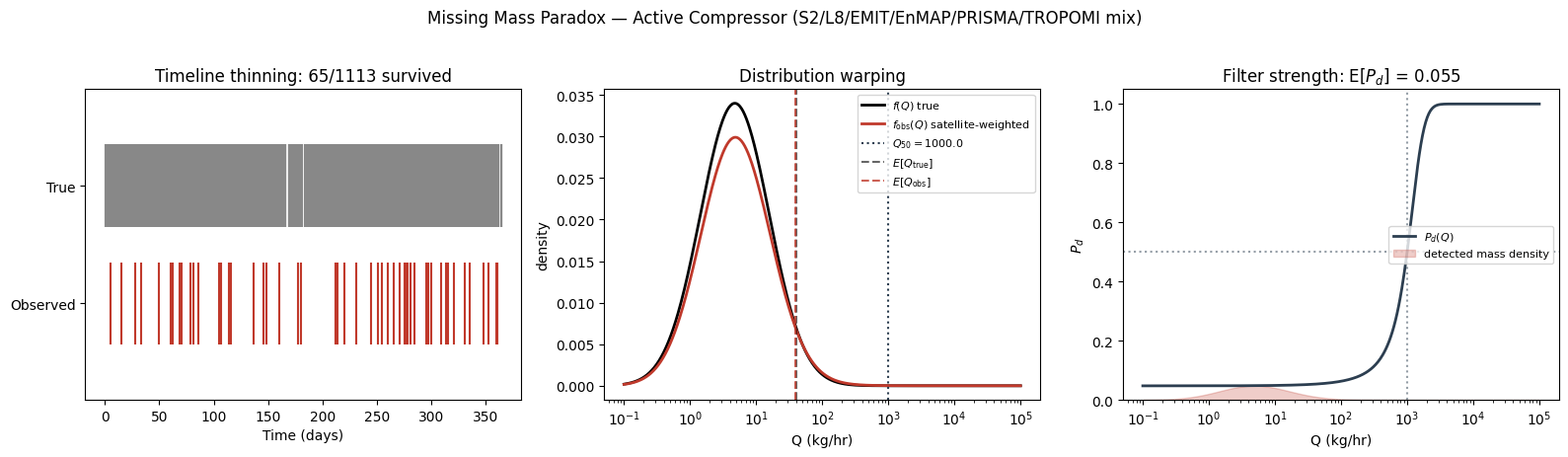

3. Why the PDFs look so similar — and where the paradox actually hides¶

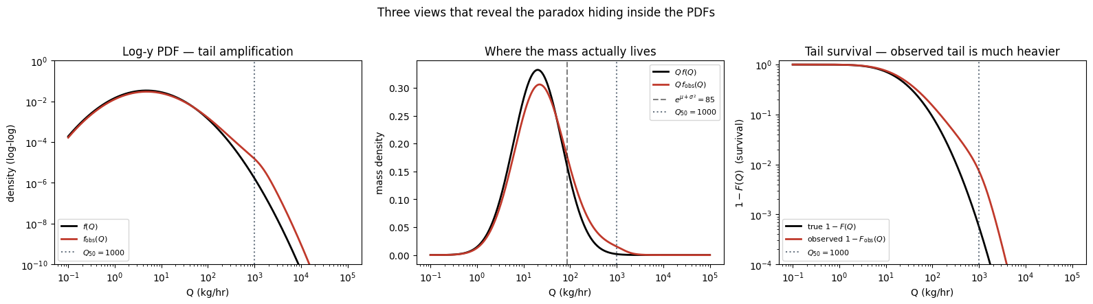
At a casual glance the true PDF $f(Q)$ and the satellite-weighted PDF $f_{\text{obs}}(Q)$ look nearly indistinguishable on the linear-y semilogx plot above. This is not a bug in the simulation; it is a real property of the realistic-constellation regime. When the POD transition sits well to the right of the bulk of the mark distribution (realistic case: $\ln Q_{50} \gg \mu$ ), then $P_d(Q)$ is a nearly-flat (small) multiplier across the Q-range where $f(Q)$ has visible probability mass. Under that condition $f_{\text{obs}}(Q) = f(Q) P_d(Q) / \mathbb{E}[P_d]$ has the same shape as $f(Q)$ in the bulk — even though the paradox is present in the numbers.

So the paradox is real, but it lives in quantities the linear-y PDF plot hides. Three views make it obvious:

Log-y PDF — at $Q \gg Q_{50}$ we have $P_d(Q) \to 1$ while $\mathbb{E}[P_d]$ stays small, giving $f_{\text{obs}}/f_{\text{true}} \to 1/\mathbb{E}[P_d]$ . That is a 10×–100× amplification of the far-right tail, completely invisible on linear-y.
Mass density $Q\,f(Q)$ — the thing you actually integrate to get total mass. The true mass peaks near $\exp(\mu+\sigma^2)$ ; the detection-weighted mass peaks out near $Q_{50}$ . The horizontal shift between the two peaks IS the paradox, visualised.
CDF — the observed CDF is visibly right-shifted against the true CDF. At the 50th percentile the gap is often an order of magnitude in Q.

from scipy.integrate import cumulative_trapezoid


mass_true = q_grid * f_true
mass_obs = q_grid * f_obs

cdf_true = cumulative_trapezoid(f_true, q_grid, initial=0.0)
cdf_true = cdf_true / cdf_true[-1]
cdf_obs = cumulative_trapezoid(f_obs, q_grid, initial=0.0)
cdf_obs = cdf_obs / cdf_obs[-1]

mu_plus_s2 = float(np.exp(cfg.mu + cfg.sigma**2))  # mass-mode of the lognormal

fig, axes = plt.subplots(1, 3, figsize=(16, 4.3))

# --- log-y PDF
ax = axes[0]
ax.loglog(q_grid, f_true, "k-", lw=2, label="$f(Q)$")
ax.loglog(q_grid, f_obs, "#c0392b", lw=2, label="$f_{\\rm obs}(Q)$")
ax.axvline(
    cfg.Q_50, color="#2c3e50", ls=":", alpha=0.7, label=f"$Q_{{50}}={cfg.Q_50:.0f}$"
)
ax.set_ylim(1e-10, 1.0)
ax.set_xlabel("Q (kg/hr)")
ax.set_ylabel("density (log-log)")
ax.set_title("Log-y PDF — tail amplification")
ax.legend(loc="lower left", fontsize=8)

# --- Mass density Q·f(Q)
ax = axes[1]
ax.semilogx(q_grid, mass_true, "k-", lw=2, label=r"$Q\,f(Q)$")
ax.semilogx(q_grid, mass_obs, "#c0392b", lw=2, label=r"$Q\,f_{\rm obs}(Q)$")
ax.axvline(
    mu_plus_s2,
    color="k",
    ls="--",
    alpha=0.5,
    label=f"$e^{{\\mu+\\sigma^2}}={mu_plus_s2:.0f}$",
)
ax.axvline(
    cfg.Q_50, color="#2c3e50", ls=":", alpha=0.7, label=f"$Q_{{50}}={cfg.Q_50:.0f}$"
)
ax.set_xlabel("Q (kg/hr)")
ax.set_ylabel("mass density")
ax.set_title("Where the mass actually lives")
ax.legend(loc="upper right", fontsize=8)

# --- Survival function 1-F(Q) on log-log
ax = axes[2]
surv_true = 1.0 - cdf_true
surv_obs = 1.0 - cdf_obs
ax.loglog(q_grid, surv_true, "k-", lw=2, label="true $1-F(Q)$")
ax.loglog(q_grid, surv_obs, "#c0392b", lw=2, label="observed $1-F_{\\rm obs}(Q)$")
ax.axvline(
    cfg.Q_50, color="#2c3e50", ls=":", alpha=0.7, label=f"$Q_{{50}}={cfg.Q_50:.0f}$"
)
ax.set_ylim(1e-4, 1.2)
ax.set_xlabel("Q (kg/hr)")
ax.set_ylabel("$1 - F(Q)$  (survival)")
ax.set_title("Tail survival — observed tail is much heavier")
ax.legend(loc="lower left", fontsize=8)

fig.suptitle("Three views that reveal the paradox hiding inside the PDFs", y=1.02)
fig.tight_layout()
plt.show()

# Percentile shifts — the paradox is strongest in the upper tail
quantiles = [0.50, 0.75, 0.90, 0.95, 0.99]
q_true_pct = np.interp(quantiles, cdf_true, q_grid)
q_obs_pct = np.interp(quantiles, cdf_obs, q_grid)

pct_rows = "\n".join(
    f"| {q * 100:4.0f}% | {qt:7.1f} | {qo:7.1f} | {qo / qt:4.2f}× |"
    for q, qt, qo in zip(quantiles, q_true_pct, q_obs_pct, strict=True)
)
Markdown(
    "**Percentile shifts in the observed distribution** — "
    "the median barely moves, but the upper tail blows up.\n\n"
    "| percentile | true Q (kg/hr) | observed Q (kg/hr) | shift factor |\n"
    "|---:|---:|---:|---:|\n" + pct_rows
)

4. The canonical scenario sweep¶

The paradox direction holds across every physically realistic regime. We sweep the six canonical scenarios from build_canonical_scenarios(): abandoned well (severe), active compressor (moderate), super-emitter (mild), extreme skew, sharp-sensor, soft-sensor. For each one we average over 20 seeds to reduce sampling noise.

scenarios = build_canonical_scenarios()


def sweep(cfg_, n=20):
    trials = [
        simulate_paradox(dataclasses.replace(cfg_, seed=cfg_.seed + i))
        for i in range(n)
    ]
    overest = np.nanmean([t.average_overestimation_ratio for t in trials])
    underest = np.nanmean([t.mass_underestimation_ratio for t in trials])
    mmsf = np.nanmedian([t.MMSF for t in trials if np.isfinite(t.MMSF)])
    return overest, underest, mmsf, trials[0].E_Pd


summary = []
for cfg_ in scenarios:
    o, u, m, e = sweep(cfg_)
    summary.append((cfg_.name, cfg_.Q_50, cfg_.mu, cfg_.sigma, o, u, m, e))

md_rows = "\n".join(
    f"| {name} | {q50:,.0f} | {mu:.1f} | {sigma:.1f} | {o:.3f} | {u:.4f} | {m:.2f} | {e:.4f} |"
    for name, q50, mu, sigma, o, u, m, e in summary
)

Markdown(
    "| scenario | $Q_{50}$ (kg hr⁻¹) | $\\mu$ | $\\sigma$ | $\\mathbb{E}[Q_{\\text{obs}}]/\\mathbb{E}[Q_{\\text{true}}]$ | $M_{\\text{obs}}/M_{\\text{true}}$ | MMSF | $\\mathbb{E}[P_d]$ |\n"
    "|---|---:|---:|---:|---:|---:|---:|---:|\n" + md_rows
)

Every scenario satisfies the two-proof structure:

Average overestimation ratio ≥ 1 (the satellite’s sample mean exceeds the true mean).
Mass underestimation ratio ≤ 1 (the satellite’s sample sum falls short of the true total).

The severity depends on where the bulk of the lognormal mark distribution sits relative to the detection threshold $Q_{50}$ . When $Q_{50}$ is far above the median mark (abandoned-well case), the satellite sees only the upper tail and the paradox is extreme. When $Q_{50}$ is at or below the median (super-emitter case), detection is near-complete and the paradox is mild.

5. Visual dashboard across scenarios¶

Six mini-panels, one per scenario, showing the mass density $Q\,f(Q)$ vs $Q\,f_{\text{obs}}(Q)$ . Using the mass density (rather than the raw PDF) makes the right-shift of the observed distribution visible in every panel — the red curve peaks near $Q_{50}$ while the black curve peaks near $\exp(\mu+\sigma^2)$ . That horizontal gap is the paradox made visible.

fig, axes = plt.subplots(2, 3, figsize=(15, 7.5), sharex=True)

for ax, cfg_ in zip(axes.flat, scenarios, strict=True):
    q = np.logspace(-1, 5, 500)
    f_t = lognormal_pdf(q, cfg_.mu, cfg_.sigma)
    pod = logistic_pod(q, cfg_.Q_50, cfg_.k)
    f_o = f_t * pod
    z = np.trapezoid(f_o, q)
    f_o = f_o / z if z > 0 else f_o

    # Mass densities
    m_t = q * f_t
    m_o = q * f_o

    ax.semilogx(q, m_t, "k-", lw=1.8, label=r"$Q\,f(Q)$")
    ax.semilogx(q, m_o, "#c0392b", lw=1.8, label=r"$Q\,f_{\rm obs}(Q)$")
    ax.axvline(
        cfg_.Q_50,
        color="#2c3e50",
        ls=":",
        alpha=0.6,
        label=f"$Q_{{50}}={cfg_.Q_50:.0f}$",
    )
    mu_mass_peak = float(np.exp(cfg_.mu + cfg_.sigma**2))
    ax.axvline(mu_mass_peak, color="k", ls="--", alpha=0.4)
    ax.set_title(cfg_.name, fontsize=9)
    ax.set_ylabel("mass density")
    e_pd = compute_E_Pd(cfg_.mu, cfg_.sigma, cfg_.Q_50, cfg_.k)
    ax.text(
        0.03,
        0.95,
        f"$E[P_d]={e_pd:.3f}$",
        transform=ax.transAxes,
        va="top",
        fontsize=9,
    )

for ax in axes[-1, :]:
    ax.set_xlabel("Q (kg/hr)")
axes[0, 0].legend(loc="center right", fontsize=8)
fig.suptitle(
    r"Mass density $Q\,f(Q)$ — true (black) vs satellite-weighted (red)", y=1.01
)
fig.tight_layout()
plt.show()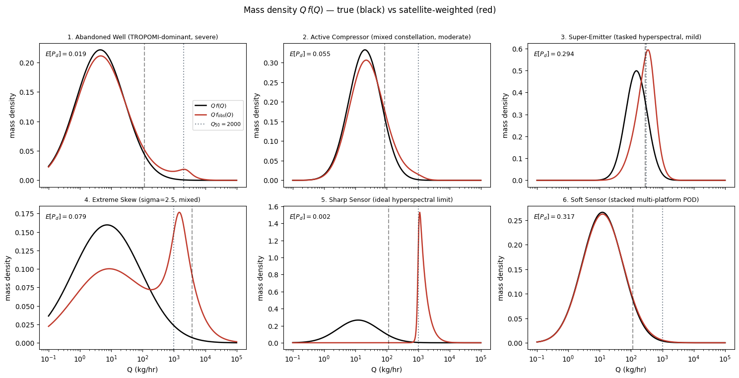

6. Sensitivity to μ and σ¶

Fix the satellite (keep $Q_{50}, k$ constant at the realistic constellation values above) and sweep the mark distribution. The heatmap below shows $E[P_d]$ — the scalar “blindness factor”. When the lognormal mean is well below the detection threshold, the satellite is nearly blind (dark region). As $\mu$ rises past $\ln Q_{50} \approx 6.9$ , the satellite becomes saturated. Larger $\sigma$ (heavier tail) raises $E[P_d]$ at fixed $\mu$ because the right tail reaches into the detectable regime, but the paradox ratios also grow because the detectable right tail carries most of the mass.

mus = np.linspace(0.5, 8.0, 25)
sigmas = np.linspace(0.5, 3.0, 25)
MU, SIGMA = np.meshgrid(mus, sigmas, indexing="ij")
E_PD = np.zeros_like(MU)

Q_50_const, k_const = 1000.0, 0.003

for i, mu in enumerate(mus):
    for j, sigma in enumerate(sigmas):
        E_PD[i, j] = compute_E_Pd(mu, sigma, Q_50=Q_50_const, k=k_const, n_quad=4000)

fig, ax = plt.subplots(figsize=(7.5, 5))
pcm = ax.pcolormesh(MU, SIGMA, E_PD, cmap="viridis", shading="auto", vmin=0, vmax=1)
cs = ax.contour(
    MU, SIGMA, E_PD, levels=[0.05, 0.1, 0.25, 0.5, 0.75], colors="white", linewidths=0.8
)
ax.clabel(cs, inline=True, fontsize=8, fmt="%.2f")
ax.axvline(
    np.log(Q_50_const), color="white", ls="--", alpha=0.8, label="$\\mu = \\ln Q_{50}$"
)
ax.set_xlabel("$\\mu$  (lognormal location)")
ax.set_ylabel("$\\sigma$  (lognormal scale)")
ax.set_title(
    f"$E[P_d]$ as a function of the mark distribution\n"
    f"(fixed $Q_{{50}}={Q_50_const:.0f}$, $k={k_const}$ — mixed constellation)"
)
ax.legend(loc="upper left")
fig.colorbar(pcm, ax=ax, label="$E[P_d]$")
fig.tight_layout()
plt.show()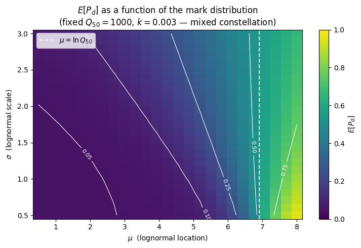

Takeaways¶

The paradox is not a bug in any particular satellite — it is a mathematical consequence of running a size-dependent filter over a heavy-tailed mark distribution.
A single scalar $E[P_d]$ governs the severity: small $E[P_d]$ means large MMSF.
Any operational inference built from satellite plume tallies must be debiased with a filter-aware model (next notebooks).
The companion notebook stationary NumPyro MCMC shows how to invert this filter via NumPyro.