Why layers: the single-slab error in v0

plumax’s forward model and its observation operator put the whole methane column in one slab at one pressure and temperature. radtrax’s v0 forward model, ForwardModel, puts it in layers. This notebook runs both on the same column and reproduces the radtrax · 3 finding: a slab at the lowest layer’s pressure misstates a band’s optical depth by up to 19 %, because it broadens every line as if all the methane sat near the surface. A slab at the column’s pressure-weighted mean does better, but is still off by 3 %.

What you’ll learn:

How to compose a layered forward model: opacity, solver, surface, geometry, instrument.
How large the single-slab error is, band by band.
How to get the matched-filter target $t = \partial \ln y / \partial \Delta X$ from the layered model by autodiff.

Background¶

Beer–Lambert along the two-way path gives the radiance at the top of the atmosphere, and a band integrates it over the instrument’s spectral response $f_b$ :

L(\nu) = \frac{E_0 \mu_0}{\pi} A \exp\Big(-m \sum_l \tau_l(\nu)\Big), \qquad y_b = \sum_g f_{bg} L(\nu_g)

(1)

with $m = 1/\mu_0 + 1/\mu$ the air-mass factor and $\tau_l = \sigma(\nu; p_l, T_l)\, n_l x_l \Delta z_l$ layer $l$ ’s optical depth. A line’s width grows with pressure, so the same column of methane absorbs differently at 1 atm and at 0.3 atm; a single slab must pick one. We compare a band’s optical depth $\tau_b = -\ln(y_b / y_b^{\text{no gas}})$ through 20 layers and through one slab holding the same column.

The cross sections are radtrax · 3’s synthetic spectrum: 150 Voigt lines near 4300 cm⁻¹, built in about a second, so the notebook runs without HITRAN. With HITRAN tables, build them with python -m radtrax.spectroscopy.hitran CH4 and load them with radtrax.spectroscopy.load_opacity.

import subprocess
import sys


try:
    import google.colab  # noqa: F401

    IN_COLAB = True
except ImportError:
    IN_COLAB = False

if IN_COLAB:
    subprocess.run(
        [
            sys.executable,
            "-m",
            "pip",
            "install",
            "-q",
            "radtrax @ git+https://github.com/jejjohnson/radtrax@main",
        ],
        check=True,
    )

import warnings


warnings.filterwarnings("ignore", message=r".*IProgress.*")

import jax


jax.config.update("jax_enable_x64", True)

import equinox as eqx
import jax.numpy as jnp
import matplotlib.pyplot as plt
import numpy as np

import radtrax
from radtrax.atmosphere import (
    ATM_TO_PA,
    AtmosphericState,
    ViewingGeometry,
)
from radtrax.instrument import BandInstrument
from radtrax.solvers import BeerLambert
from radtrax.spectroscopy import TableOpacity
from radtrax.spectroscopy.synthetic import NU_CM as NU, synthetic_table
from radtrax.surface import Lambertian

import importlib.util


try:
    from IPython import get_ipython

    ipython = get_ipython()
except ImportError:
    ipython = None

if ipython is not None and importlib.util.find_spec("watermark") is not None:
    ipython.run_line_magic("load_ext", "watermark")
    ipython.run_line_magic("watermark", "-v -m -p numpy,jax,equinox,radtrax")
else:
    print("watermark extension not installed; skipping reproducibility readout.")

Python implementation: CPython
Python version       : 3.13.5
IPython version      : 9.10.0

numpy  : 2.4.4
jax    : 0.11.2
equinox: 0.13.8
radtrax: 0.0.0

Compiler    : GCC 11.2.0
OS          : Linux
Release     : 6.8.0-1044-azure
Machine     : x86_64
Processor   : x86_64
CPU cores   : 16
Architecture: 64bit

1. The cross-section table¶

σ(ν; T, p) on 4230–4370 cm⁻¹ at 0.01 cm⁻¹, ten pressures (0.03–1.1 atm) and six temperatures (200–310 K): line strengths log-normal at 296 K, Lorentz widths $\gamma_{\text{air}} (p / 1\,\text{atm}) (296/T)^{0.75}$ , Doppler widths of CH₄. The format is the one radtrax.spectroscopy.hitran writes. It is radtrax · 3’s own code, radtrax.spectroscopy.synthetic.synthetic_table, the same table radtrax’s tests use.

table = synthetic_table(seed=0)  # σ(ν; T, p) on NU, T and p

2. The forward model¶

TableOpacity interpolates σ bilinearly in $(\ln p, T)$ for each layer, BeerLambert gives the radiance, and BandInstrument integrates seven Gaussian bands, 8.5 nm wide and 14 cm⁻¹ apart, as in radtrax · 3.

centres = np.arange(4257.0, 4345.0, 14.0)  # cm⁻¹                          (B,)
# An 8.5 nm FWHM is ν² Δλ / 10⁷ in wavenumber: 15.7 cm⁻¹ at 4300 cm⁻¹.
fwhm_cm = centres**2 * 8.5 / 1e7
sd_cm = fwhm_cm / (2 * np.sqrt(2 * np.log(2)))
response = np.exp(-0.5 * ((NU[None] - centres[:, None]) / sd_cm[:, None]) ** 2)
response /= response.sum(axis=1, keepdims=True)  # each row sums to 1   (B, G)

model = radtrax.ForwardModel(
    TableOpacity.from_datasets({"CH4": table}),
    BeerLambert(),
    BandInstrument(NU, response),
)
geometry = ViewingGeometry.from_angles(35.0, 0.0)
surface = Lambertian(1.0)

3. Twenty layers against one slab¶

Twenty one-kilometre layers with an 8 km scale height and a 6.5 K/km lapse rate down to 217 K, holding 1.9 ppm of methane. The two slabs hold the same column, at the lowest layer’s $(p, T)$ (0.94 atm, 285 K) and at the column’s air-weighted mean $(p, T)$ .

z_km = np.arange(0.5, 20.0, 1.0)  # layer middles                        (L,)
p_atm = np.exp(-z_km / 8.0)
t_k = np.maximum(288.0 - 6.5 * z_km, 217.0)
X0 = 1.9e-6


def state(p_atm, t_k, z_m, dz_m, vmr) -> AtmosphericState:
    return AtmosphericState(
        p_pa=jnp.asarray(p_atm * ATM_TO_PA),
        t_k=jnp.asarray(t_k),
        z_m=jnp.asarray(z_m),
        dz_m=jnp.asarray(dz_m),
        vmr={"CH4": jnp.asarray(vmr)},
    )


layered = state(p_atm, t_k, 1000.0 * z_km, np.full(20, 1000.0), np.full(20, X0))
column = float(layered.column("CH4"))  # molecules/cm²
weights = np.asarray(layered.air_column())
weights = weights / weights.sum()


def slab_at(p, t) -> AtmosphericState:
    p, t, x = np.array([p]), np.array([t]), np.array([X0])
    one = state(p, t, np.array([500.0]), np.array([1000.0]), x)
    dz_m = 1000.0 * column / float(one.column("CH4"))  # the same column
    return state(p, t, np.array([dz_m / 2]), np.array([dz_m]), x)


@eqx.filter_jit
def band_tau(atm: AtmosphericState) -> jax.Array:
    # τ_b = −ln(y_b / y_b(no gas))                                        (B,)
    clear = model(atm.with_vmr("CH4", 0.0), surface, geometry)
    return -jnp.log(model(atm, surface, geometry) / clear)


tau_layers = np.asarray(band_tau(layered))
tau_surface = np.asarray(band_tau(slab_at(p_atm[0], t_k[0])))
mean_p, mean_t = (weights * p_atm).sum(), (weights * t_k).sum()
tau_mean = np.asarray(band_tau(slab_at(mean_p, mean_t)))
print(f"CH₄ column: {column:.3g} molecules/cm²")
err = np.max(np.abs(tau_surface / tau_layers - 1))
print(f"lowest-layer slab: up to {err:.1%} off")
print(f"mean slab:    up to {np.max(np.abs(tau_mean / tau_layers - 1)):.1%} off")

CH₄ column: 4.1e+19 molecules/cm²
lowest-layer slab: up to 18.6% off
mean slab:    up to 3.1% off

fig, ax = plt.subplots(figsize=(12, 5))
for tau, label in [
    (tau_surface, "slab at the lowest layer"),
    (tau_mean, "slab at the mean (p, T)"),
]:
    ax.plot(centres, 100 * (tau / tau_layers - 1), "o-", label=label)
ax.axhline(0.0, color="k", linestyle="--", label="20 layers")
ax.set_xlabel("band centre [cm⁻¹]")
ax.set_ylabel("band optical depth vs 20 layers [%]")
ax.legend()
plt.show()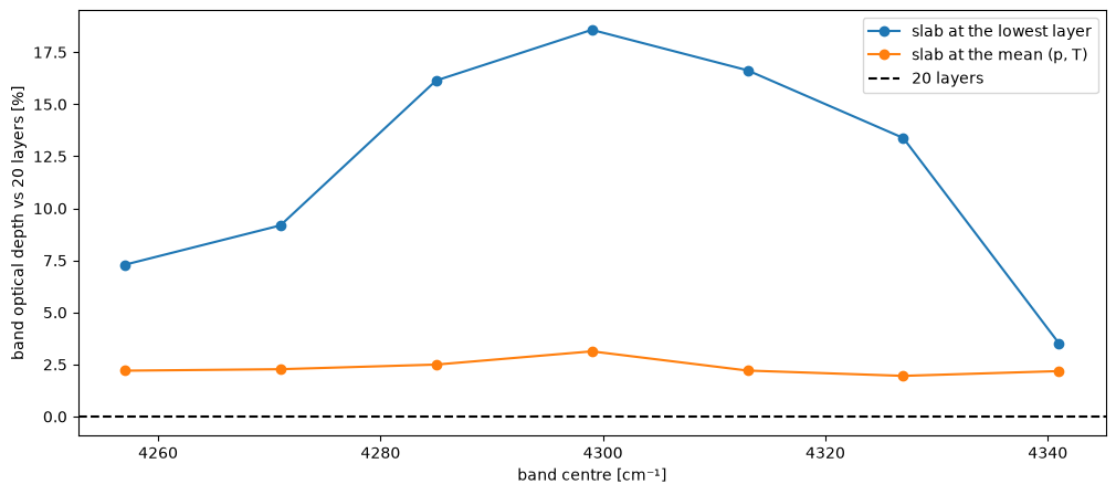

The slab at the lowest layer broadens every line as if all the methane sat near the surface. Its band optical depth is off by up to 19 %. The slab at the mean $(p, T)$ is off by up to 3 %. That is an error of the model’s structure, and it is 30 times the 0.1 % to which v0 holds its tables’ interpolation. The layers are not decoration: they are the first thing v0 changes.

4. The matched-filter target from autodiff¶

unit_absorption_target differentiates $\ln y$ with respect to a column enhancement $\Delta X$ [mol/m²], here spread over the lowest kilometre, by one forward-mode pass. It depends on the scene through the state and the geometry, which is why a target per scene replaces a MODTRAN table. The slab’s target is off too, by up to 3.8 % here: a smaller error than in the optical depth, because the plume itself sits in the lowest kilometre, near the surface’s pressure.

target = eqx.filter_jit(radtrax.unit_absorption_target)
t_layers = np.asarray(target(model, layered, surface, geometry))
slab = slab_at(p_atm[0], t_k[0])
t_slab = np.asarray(target(model, slab, surface, geometry))
print("t, 20 layers [per mol/m²]:", np.round(t_layers, 4))
err = np.max(np.abs(t_slab / t_layers - 1))
print(f"lowest-layer slab: up to {err:.1%} off")

t, 20 layers [per mol/m²]: [-0.0427 -0.035  -0.0526 -0.0845 -0.0692 -0.0616 -0.0634]
lowest-layer slab: up to 3.8% off

Summary¶

ForwardModel(opacity, solver, instrument)(state, surface, geometry) gives one value per band, and every input is differentiable.
Through one slab at the lowest layer’s $(p, T)$ , a band’s optical depth is off by up to 19 % (18.6 %) from 20 layers; at the column’s mean $(p, T)$ , by up to 3 % (3.1 %).
The slab’s matched-filter target is off by up to 3.8 %.
unit_absorption_target gives each scene its own matched-filter target, $t = \partial \ln y / \partial \Delta X$ .