Duration? Mean of Globe -> Correlated with Mean Location of Extremes Metrics ¶ Log-Likelihood ¶ Table 1: Table with results for each model
Model NLL Error IID Model-17089.15032017 4.06643326 Spatial Model -16663.58281494 62.91590443 Temporal Model -15571.70729426 4.73258625 Spatiotemporal Model -15198.35183499 59.1095967
Figure 2: (5)
Figure 2: (5)
Figure 2: (5)
Figure 2: (5)
Parameters ¶ Location Parameter ¶ For the location parameter, recall the formulation
μ ( t , s , θ ) = μ 0 + μ 1 t + μ 2 ( s ) \boldsymbol{\mu}(t,\mathbf{s},\boldsymbol{\theta}) =
\mu_0 +
\mu_1t +
\mu_2(\mathbf{s}) μ ( t , s , θ ) = μ 0 + μ 1 t + μ 2 ( s ) So for this experiment, each model has a location bias parameter, μ 0 \mu_0 μ 0 and the location-temporal weight parameter, μ 1 \mu_1 μ 1
Location-Bias ¶ Histogram ¶ This is the histogram of all samples of the location-bias parameter, μ 0 \mu_0 μ 0
Figure 2: (5)
Figure 2: (5)
Figure 2: (5)
Mean Histogram ¶ This is the histogram of the mean of the location-bias parameter, μ 0 \mu_0 μ 0
Figure 2: (5)
Figure 2: (5)
Figure 2: (5)
Maps ¶ Figure 2: (5)
Figure 2: (5)
Figure 2: (5)
Location Time-Weight ¶ We will look at the location temporal-weight parameter, μ 1 \mu_1 μ 1
Histogram ¶ Figure 2: (5)
Figure 2: (5)
Mean Histogram ¶ Figure 2: (5)
Figure 2: (5)
Maps ¶ Figure 2: (5)
Figure 2: (5)
Scale ¶ Recall, the parameterization for the scale parameter is given by
σ ( t ; θ ) = σ 0 \sigma(t;\boldsymbol{\theta})
=
\sigma_0 σ ( t ; θ ) = σ 0 where σ 0 \sigma_0 σ 0
Histogram ¶ Figure 2: (5)
Figure 2: (5)
Figure 2: (5)
Mean Histogram ¶ Figure 2: (5)
Figure 2: (5)
Figure 2: (5)
Map ¶ Figure 2: (5)
Figure 2: (5)
Figure 2: (5)
Concentration ¶ Recall, the parameterization for the shape parameter is given by
κ ( t ; θ ) = κ 0 \kappa(t;\boldsymbol{\theta})
=
\kappa_0 κ ( t ; θ ) = κ 0 where κ 0 \kappa_0 κ 0
Histogram ¶ Figure 2: (5)
Figure 2: (5)
Figure 2: (5)
Mean Histogram ¶ Figure 2: (5)
Figure 2: (5)
Figure 2: (5)
Maps ¶ Figure 2: (5)
Figure 2: (5)
Figure 2: (5)
Rate ¶ We can relate the GEVD parameters to the GPD .
This gives us a rate parameter, λ, which is the expected number of events that exceed some threshold, y 0 y_0 y 0
λ = σ + κ ( y 0 − μ ) \lambda = \sigma + \kappa (y_0 - \mu) λ = σ + κ ( y 0 − μ ) However, we need to define an exceedence threshold, y 0 y_0 y 0
Threshold ¶ Figure 38: y 0 y_0 y 0
Figure 39: y 0 y_0 y 0
Histogram ¶ Figure 2: (5)
Figure 2: (5)
Figure 2: (5)
Mean Histogram ¶ Figure 2: (5)
Figure 2: (5)
Figure 2: (5)
Maps ¶ GMST - Scenario 0¶ Figure 2:
Figure 2: GMST scenario 0 for the temporal model.
Figure 2: GMST scenario 0 for the spatio-temporal model.
GMST - Scenario 1¶ Figure 2:
Figure 2: GMST scenario 1 for the temporal model.
Figure 2: GMST scenario 1 for the spatio-temporal model.
GMST - Scenario 2¶ Figure 2:
Figure 2: GMST scenario 2 for the temporal model.
Figure 2: GMST scenario 2 for the spatio-temporal model.
Returns ¶ Histogram ¶ Figure 2: (5)
Figure 2: (5)
Figure 2: (5)
Figure 2: (5)
Mean Histogram ¶ Figure 2: (5)
Figure 2: (5)
Figure 2: (5)
Figure 2: (5)
Maps ¶ GMST - Scenario 0¶ Figure 2:
Figure 2: GMST scenario 0 for the temporal model.
Figure 2: GMST scenario 0 for the temporal model.
Figure 2: GMST scenario 0 for the spatio-temporal model.
GMST - Scenario 1¶ Figure 2:
Figure 2: GMST scenario 0 for the temporal model.
Figure 2: GMST scenario 1 for the temporal model.
Figure 2: GMST scenario 1 for the spatio-temporal model.
GMST - Scenario 2¶ Figure 2:
Figure 2: GMST scenario 0 for the temporal model.
Figure 2: GMST scenario 2 for the temporal model.
Figure 2: GMST scenario 2 for the spatio-temporal model.
Differences ¶ Case I - Scenario 0 and 1 ¶ The first case, we look at the absolute difference between the GMST scenarios 0 and 1.
This corresponds to the difference in the pre-industrial climate and the actual climate.
Figure 2: (5)
Figure 2: (5)
Case I - Scenario 1 and 2s ¶ The first case, we look at the absolute difference between the GMST scenarios 1 and 2.
This corresponds to the difference in the actual climate and the future climate.
Figure 2: (5)
Figure 2: (5)
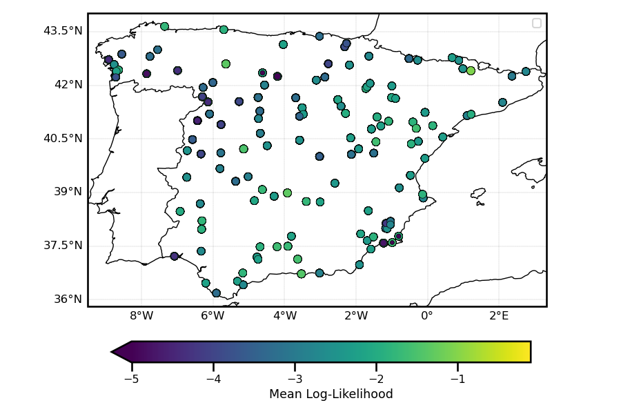 The negative log-likelihood loss (equation (5)) for each time step within the time series.
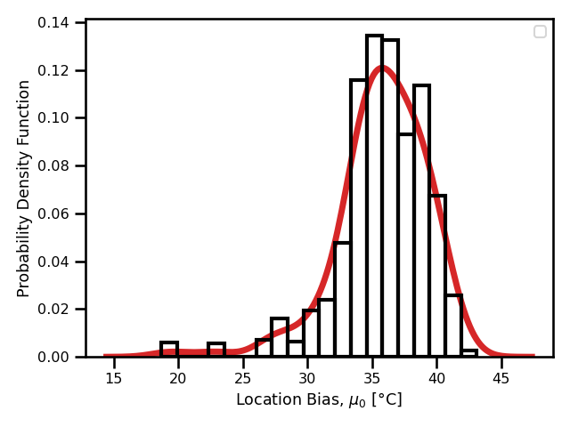 The negative log-likelihood loss (equation
 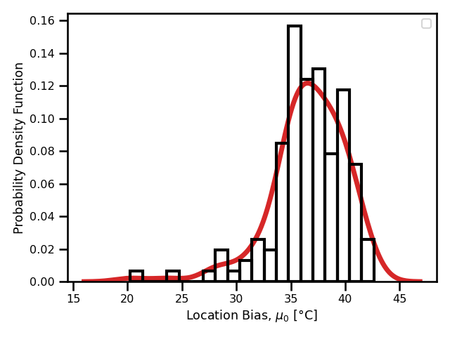 The negative log-likelihood loss (equation
 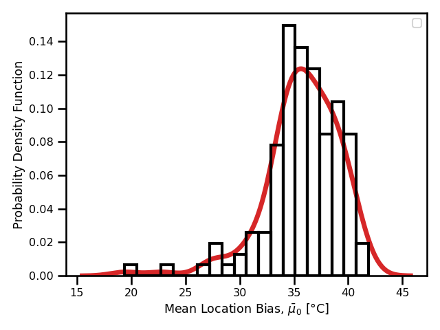 The negative log-likelihood loss (equation
 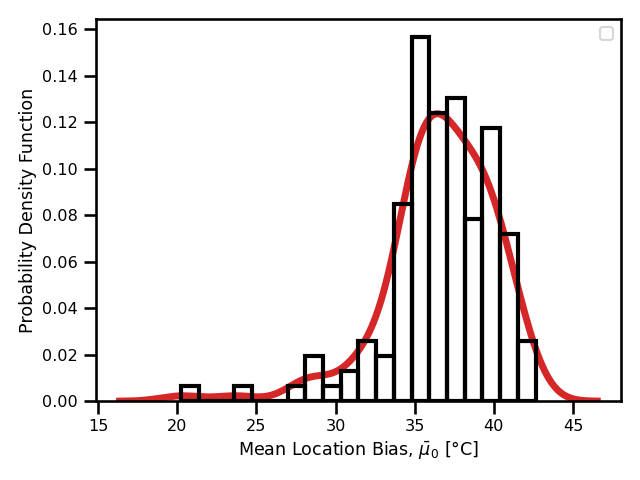 The negative log-likelihood loss (equation
 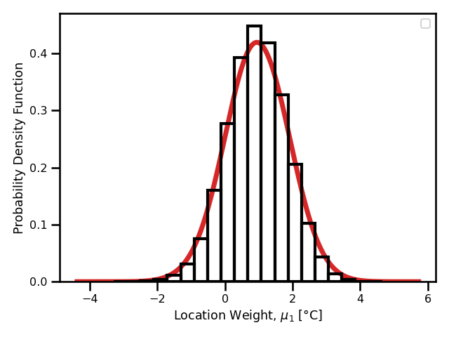 The negative log-likelihood loss (equation
 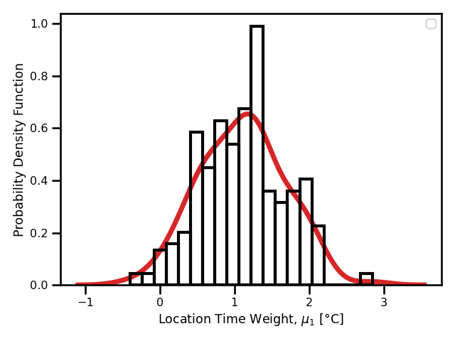 The negative log-likelihood loss (equation
 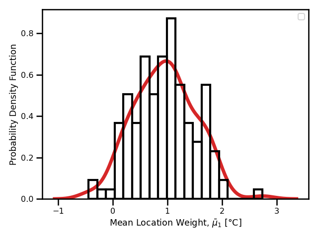 The negative log-likelihood loss (equation
 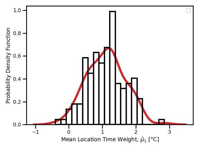 The negative log-likelihood loss (equation
 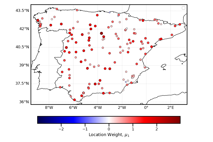 The negative log-likelihood loss (equation
 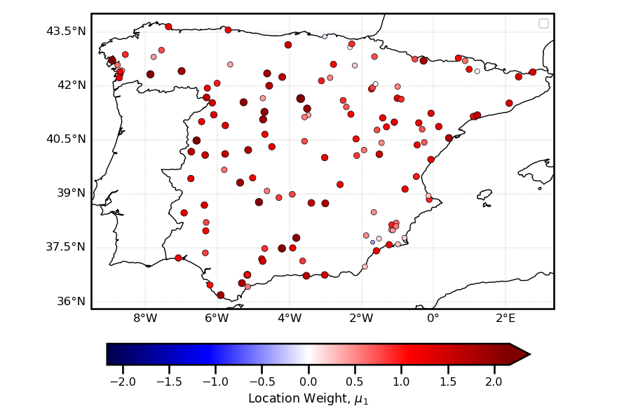 The negative log-likelihood loss (equation
 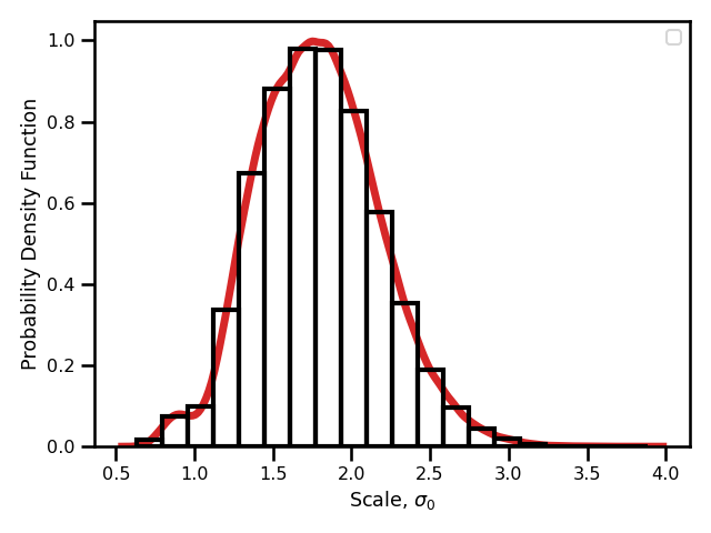 The negative log-likelihood loss (equation
 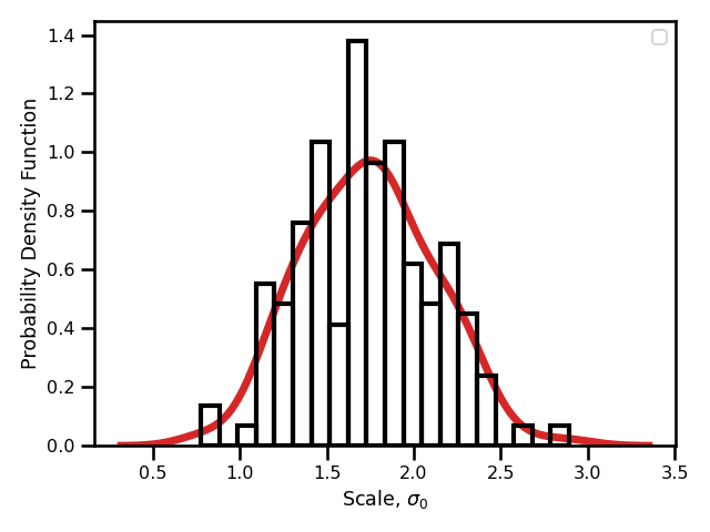 The negative log-likelihood loss (equation
 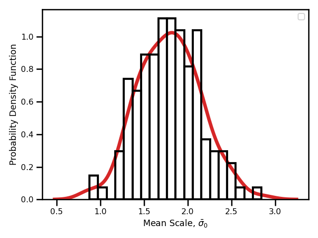 The negative log-likelihood loss (equation
 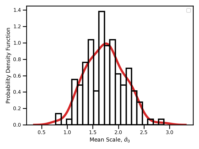 The negative log-likelihood loss (equation
 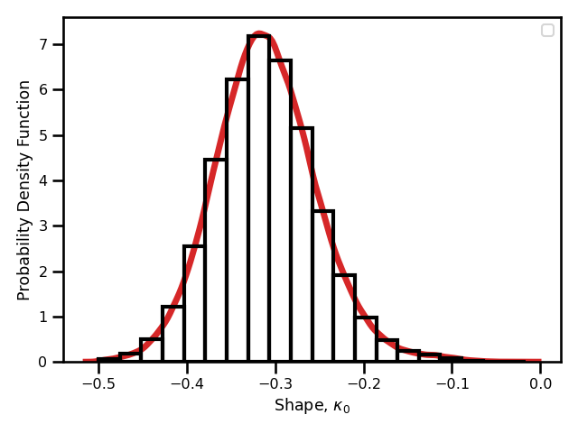 The negative log-likelihood loss (equation
 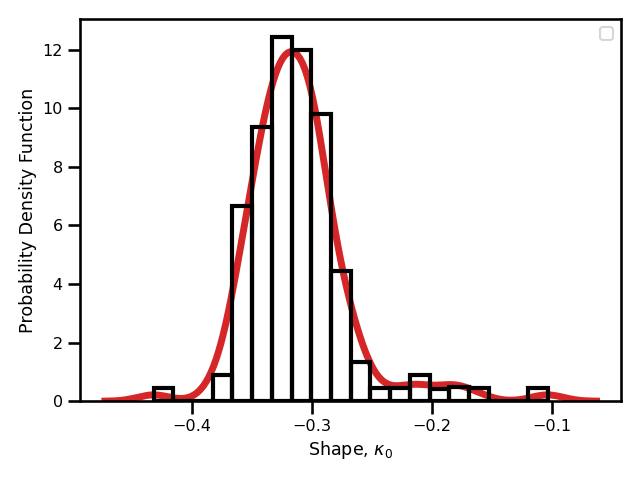 The negative log-likelihood loss (equation
 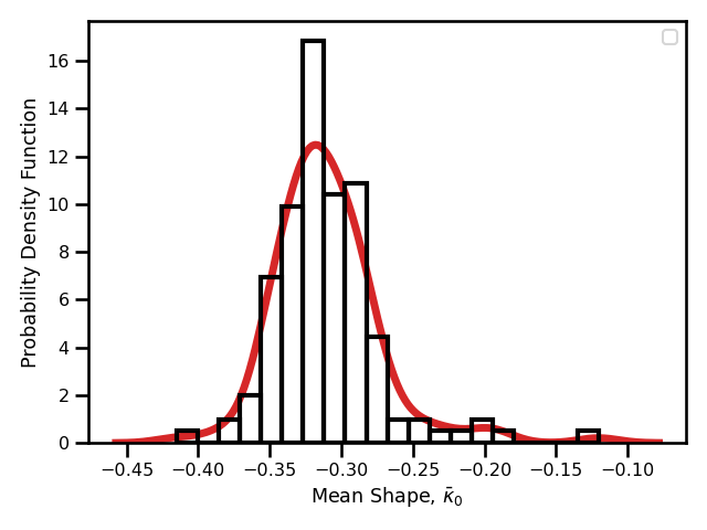 The negative log-likelihood loss (equation
 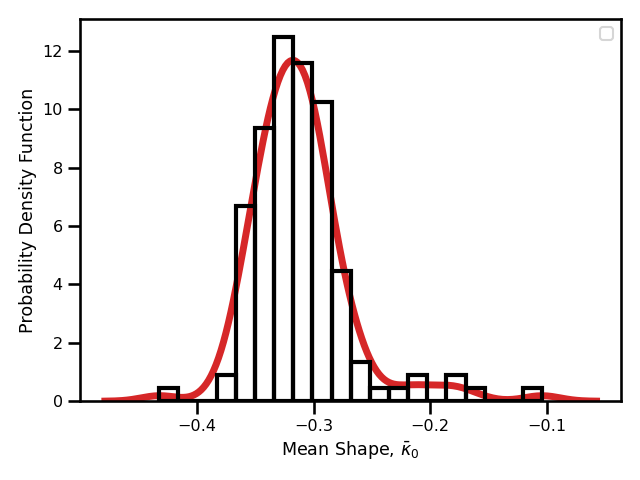 The negative log-likelihood loss (equation
 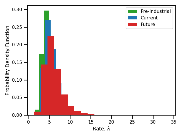 The negative log-likelihood loss (equation
 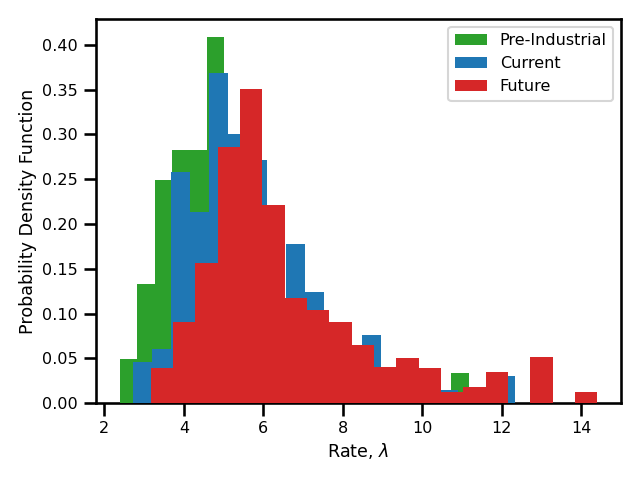 The negative log-likelihood loss (equation
 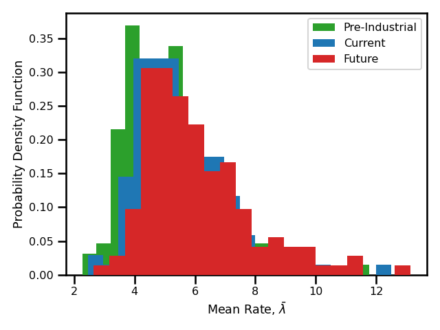 The negative log-likelihood loss (equation
 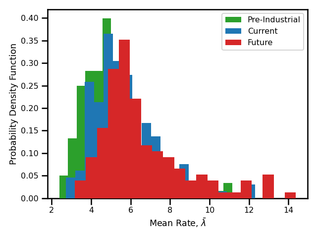 The negative log-likelihood loss (equation
 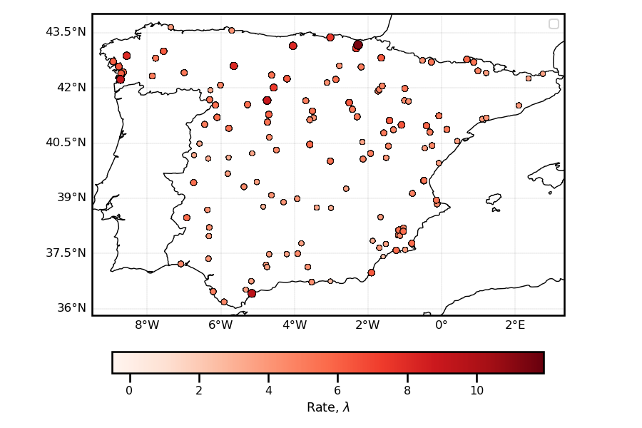 The return period under a GMST scenario 0 for the temporal model.
 The return period under a GMST scenario 0 for the spatio-temporal model.
 The return period under a GMST scenario 1 for the temporal model.
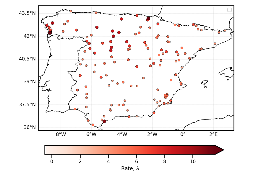 The return period under a GMST scenario 1 for the spatio-temporal model.
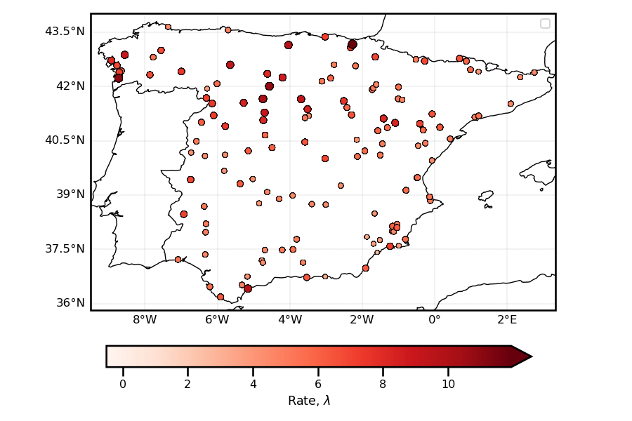 The return period under a GMST scenario 2 for the temporal model.
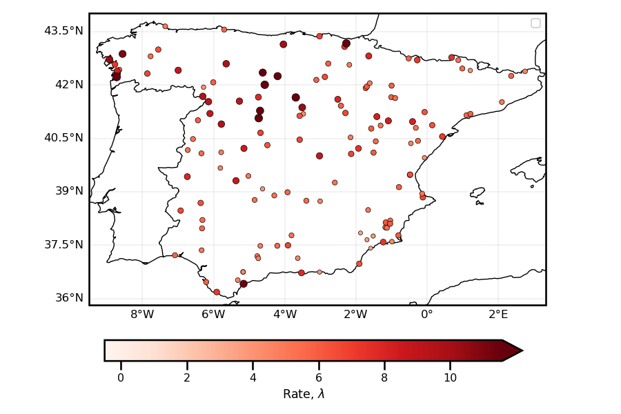 The return period under a GMST scenario 2 for the spatio-temporal model.
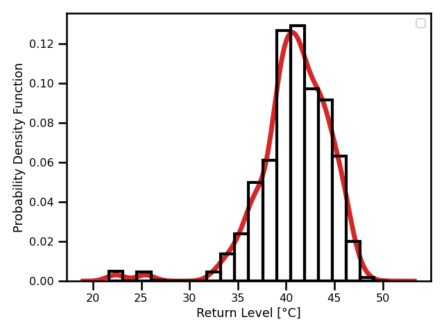 The negative log-likelihood loss (equation (5)) for each time step within the time series.
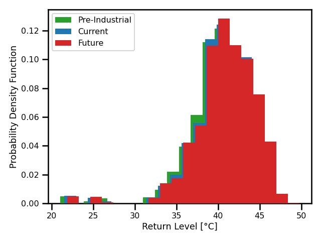 The negative log-likelihood loss (equation
 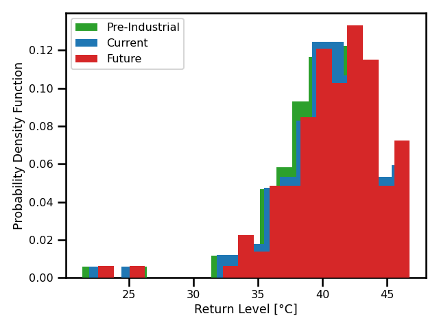 The negative log-likelihood loss (equation
 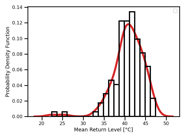 The negative log-likelihood loss (equation (5)) for each time step within the time series.
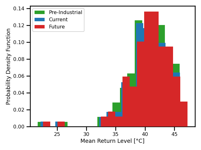 The negative log-likelihood loss (equation
  The negative log-likelihood loss (equation
 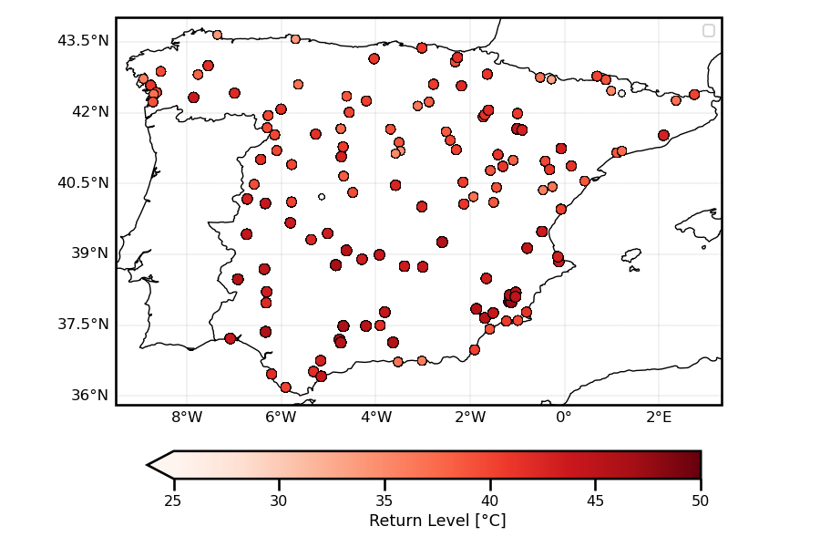 The return period under a GMST scenario 0 for the temporal model.
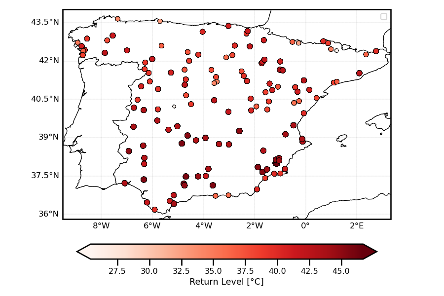 The return period under a GMST scenario 0 for the temporal model.
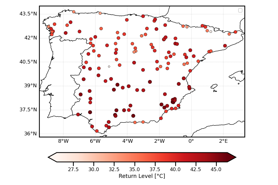 The return period under a GMST scenario 0 for the spatio-temporal model.
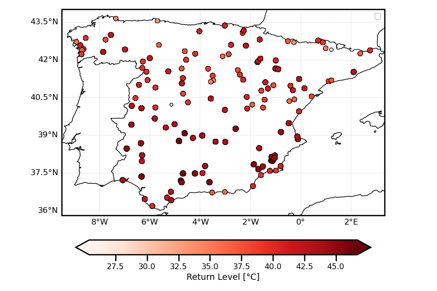 The return period for the iid model.
 The return period under a GMST scenario 1 for the spatio-temporal model.
 The return period under a GMST scenario 2 for the temporal model.
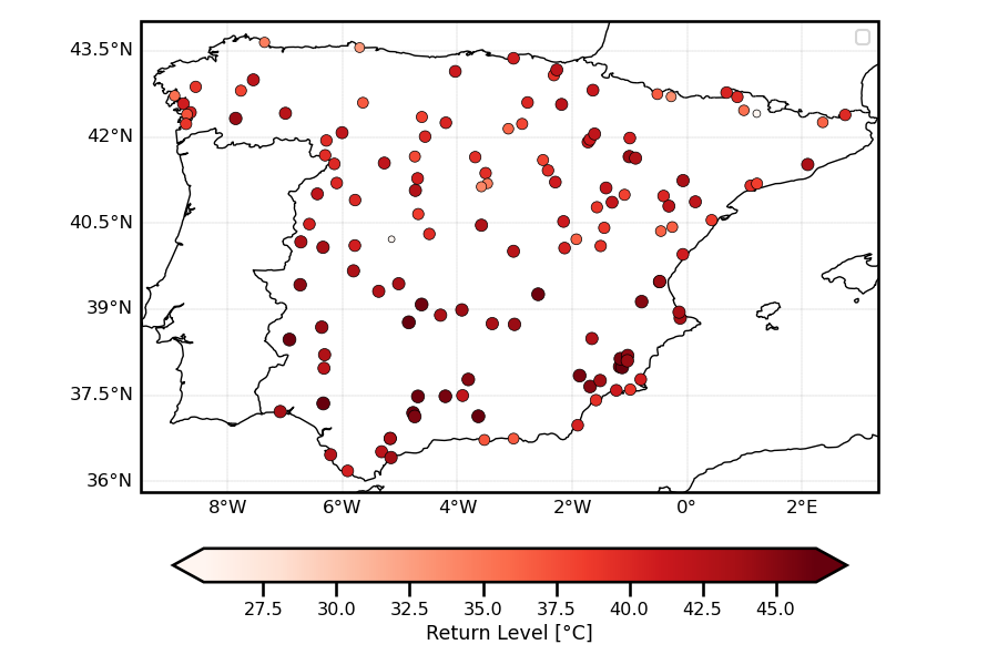 The return period under a GMST scenario 2 for the spatio-temporal model.