Duration? Mean of Globe -> Correlated with Mean Location of Extremes Metrics ¶ Log-Likelihood ¶ Table 1: Table with results for each model
Model NLL Error GEVD -124.7383235 4.06643326 GPD (Q95, 3D)-1358.70624244 20.17945954 GPD (Q98, 3D)-567.97480681 14.90358918 GPD (Q99, 3D)-291.28153454 11.48212622
GEVD
GPD (Q95, 3D)
GPD (Q95, 3D)
GPD (Q98, 3D)
GPD (Q99, 3D)
Figure 2: (5)
Figure 2: (5)
Figure 2: (5)
Figure 2: (5)
Figure 2: (5)
Parameters ¶ Location Parameter ¶ For the location parameter, recall the formulation
μ ( s , θ ) = μ 0 \boldsymbol{\mu}(\mathbf{s},\boldsymbol{\theta}) =
\mu_0 μ ( s , θ ) = μ 0 So for this experiment, each model has a location bias parameter, μ 0 \mu_0 μ 0 and the location-temporal weight parameter, μ 1 \mu_1 μ 1
Location-Bias ¶ Histogram ¶ This is the histogram of all samples of the location-bias parameter, μ 0 \mu_0 μ 0
GEVD
GPD (Q90, 3D)
GPD (Q95, 3D)
GPD (Q98, 3D)
GPD (Q98, 3D)
Figure 2: (5)
Figure 2: (5)
Figure 2: (5)
Figure 2: (5)
Figure 2: (5)
Mean Histogram ¶ This is the histogram of the mean of the location-bias parameter, μ 0 \mu_0 μ 0
GEVD
GPD (Q90, 3D)
GPD (Q95, 3D)
GPD (Q98, 3D)
GPD (Q98, 3D)
Figure 2: (5)
Figure 2: (5)
Figure 2: (5)
Figure 2: (5)
Figure 2: (5)
Maps ¶ GEVD
GPD (Q95, 3D)
GPD (Q95, 3D)
GPD (Q98, 3D)
GPD (Q98, 3D)
Figure 2: (5)
Figure 2: (5)
Figure 2: (5)
Figure 2: (5)
Figure 2: (5)
Sigma ¶ σ ∗ = σ + κ ( y 0 − μ ) \sigma^* = \sigma + \kappa (y_0 - \mu) σ ∗ = σ + κ ( y 0 − μ ) This parameter is only present for the GPD distribution.
Histogram ¶ GPD (Q95, 3D)
GPD (Q98, 3D)
Figure 2: (5)
Figure 2: (5)
Mean Histogram ¶ GPD (Q98,3D)
GPD (Q98, 3D)
Figure 2: (5)
Figure 2: (5)
Map ¶ GPD (Q95, 3D)
GPD (Q98, 3D)
Figure 2: (5)
Figure 2: (5)
Scale ¶ Recall, the parameterization for the scale parameter is given by
σ ( t ; θ ) = σ 0 \sigma(t;\boldsymbol{\theta})
=
\sigma_0 σ ( t ; θ ) = σ 0 where σ 0 \sigma_0 σ 0
Histogram ¶ GEVD
GPD (Q95, 3D)
GPD (Q98, 3D)
Figure 2: (5)
Figure 2: (5)
Figure 2: (5)
Mean Histogram ¶ GEVD
GPD (Q95, 3D)
GPD (Q98, 3D)
Figure 2: (5)
Figure 2: (5)
Figure 2: (5)
Map ¶ GEVD
GPD (Q95, 3D)
GPD (Q95, 3D)
Figure 2: (5)
Figure 2: (5)
Figure 2: (5)
Concentration ¶ Recall, the parameterization for the shape parameter is given by
κ ( t ; θ ) = κ 0 \kappa(t;\boldsymbol{\theta})
=
\kappa_0 κ ( t ; θ ) = κ 0 where κ 0 \kappa_0 κ 0
Histogram ¶ Figure 2: (5)
Figure 2: (5)
Mean Histogram ¶ GEVD
GPD (Q95, 3D)
GPD (Q98, 3D)
Figure 2: (5)
Figure 2: (5)
Figure 2: (5)
Maps ¶ GEVD
GPD (Q95, 3D)
GPD (Q98, 3D)
Figure 2: (5)
Figure 2: (5)
Figure 2: (5)
Rate ¶ We can relate the GEVD parameters to the GPD .
This gives us a rate parameter, λ, which is the expected number of events that exceed some threshold, y 0 y_0 y 0
λ = σ + κ ( y 0 − μ ) \lambda = \sigma + \kappa (y_0 - \mu) λ = σ + κ ( y 0 − μ ) However, we need to define an exceedence threshold, y 0 y_0 y 0
Threshold ¶ Figure 38: y 0 y_0 y 0
Histogram ¶ Figure 2: (5)
Mean Histogram ¶ Figure 2: (5)
Maps ¶ Figure 2:
Returns ¶ Histogram ¶ GEVD
GPD (Q90, 3D)
GPD (Q95, 3D)
GPD (Q98, 3D)
GPD (Q99, 3D)
Figure 2: (5)
Figure 2: (5)
Figure 2: (5)
Figure 2: (5)
Figure 2: (5)
Mean Histogram ¶ GEVD
GPD (Q90, 3D)
GPD (Q95, 3D)
GPD (Q98, 3D)
GPD (Q99, 3D)
Figure 2: (5)
Figure 2: (5)
Figure 2: (5)
Figure 2: (5)
Figure 2: (5)
Maps ¶ GEVD
GPD (Q90, 3D)
GPD (Q95, 3D)
GPD (Q95, 3D)
GPD (Q99, 3D)
Figure 2:
Figure 2:
Figure 2:
Figure 2:
Figure 2:
 The negative log-likelihood loss (equation (5)) for each time step within the time series.
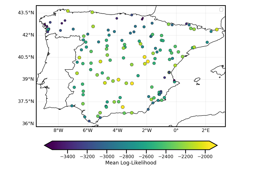 The negative log-likelihood loss (equation (5)) for each time step within the time series.
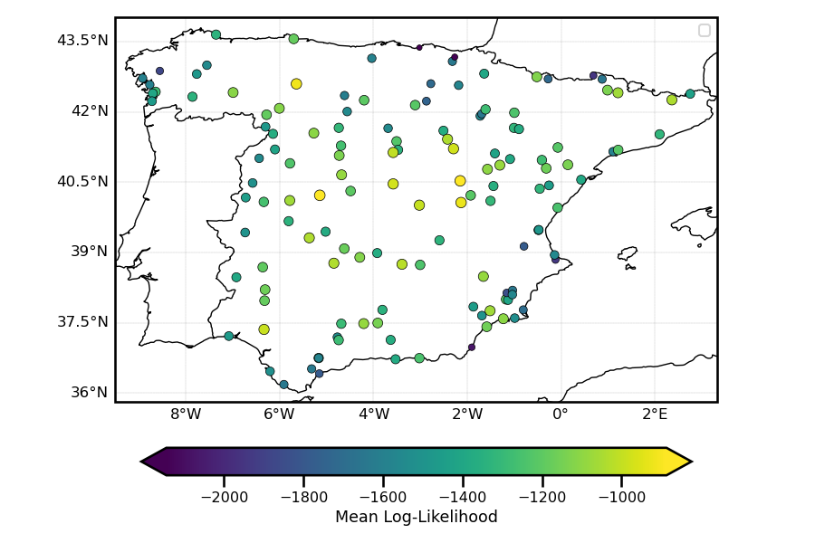 The negative log-likelihood loss (equation (5)) for each time step within the time series.
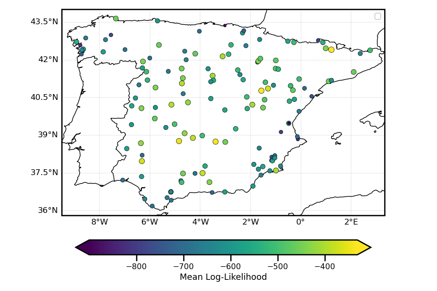 The negative log-likelihood loss (equation
  The negative log-likelihood loss (equation
 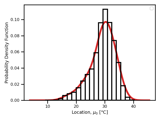 The negative log-likelihood loss (equation (5)) for each time step within the time series.
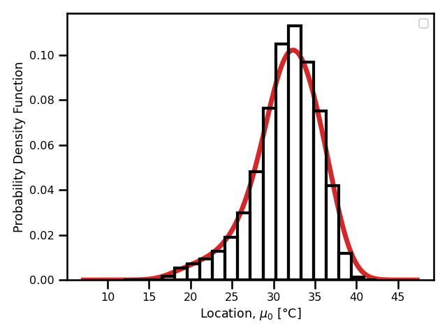 The negative log-likelihood loss (equation (5)) for each time step within the time series.
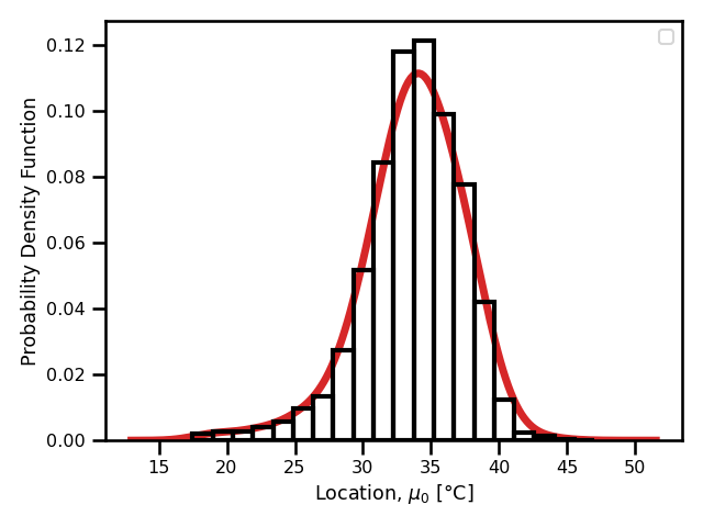 The negative log-likelihood loss (equation
 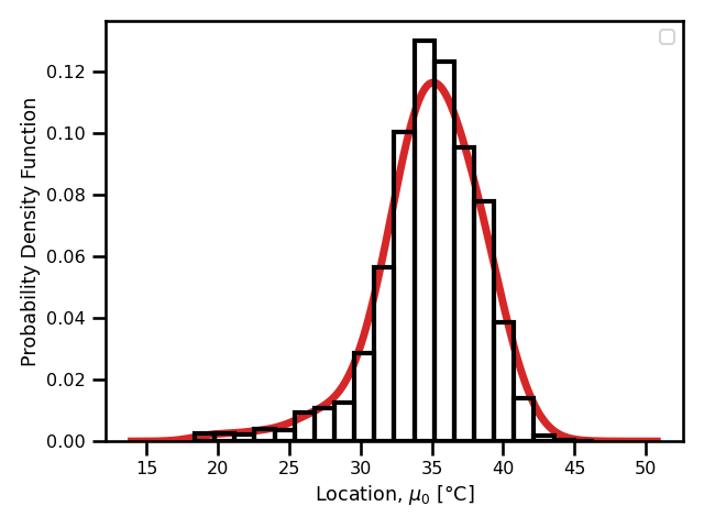 The negative log-likelihood loss (equation
 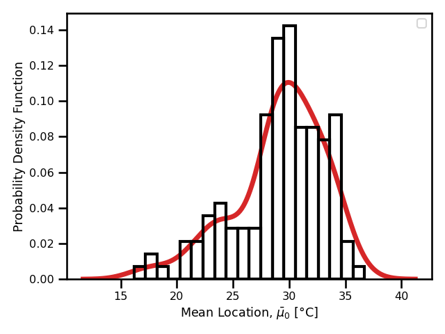 The negative log-likelihood loss (equation (5)) for each time step within the time series.
 The negative log-likelihood loss (equation (5)) for each time step within the time series.
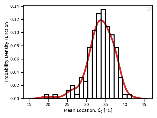 The negative log-likelihood loss (equation
 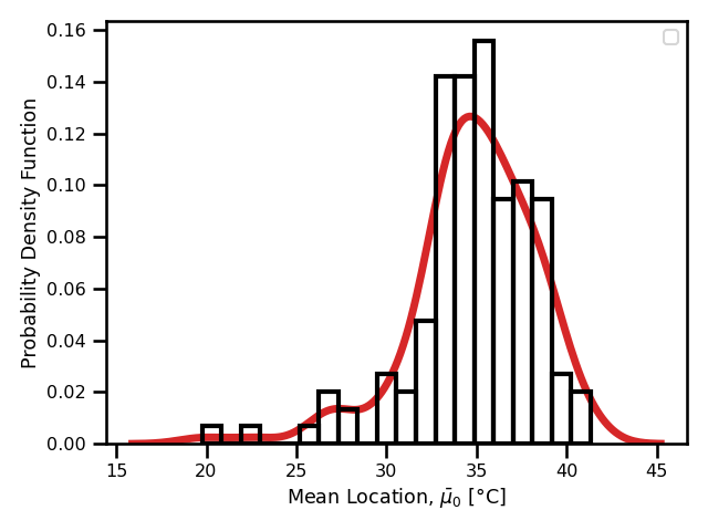 The negative log-likelihood loss (equation
  The negative log-likelihood loss (equation (5)) for each time step within the time series.
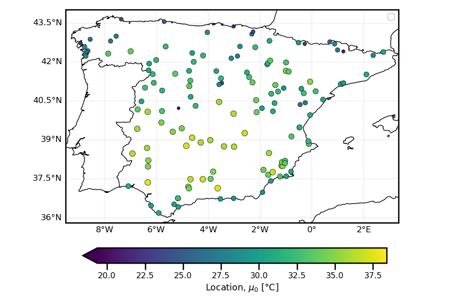 The negative log-likelihood loss (equation (5)) for each time step within the time series.
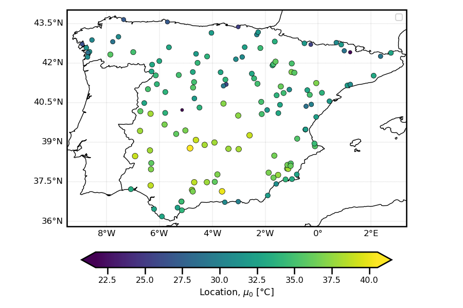 The negative log-likelihood loss (equation
 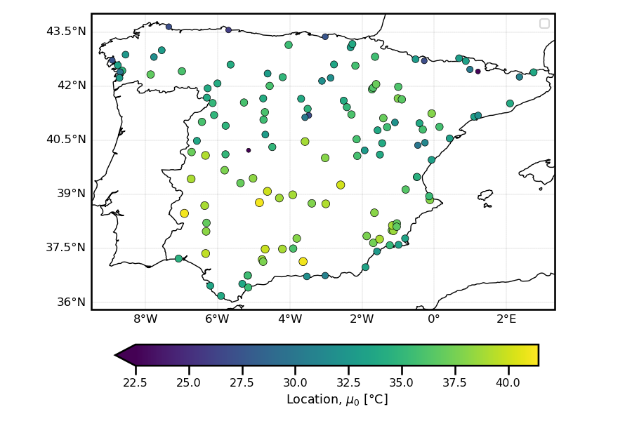 The negative log-likelihood loss (equation
 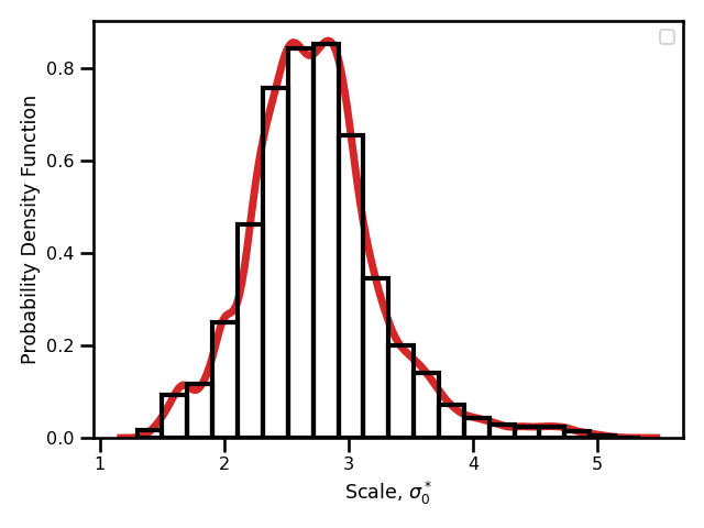 The negative log-likelihood loss (equation
 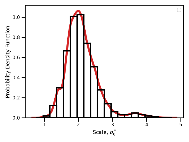 The negative log-likelihood loss (equation
 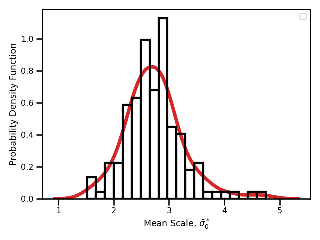 The negative log-likelihood loss (equation
 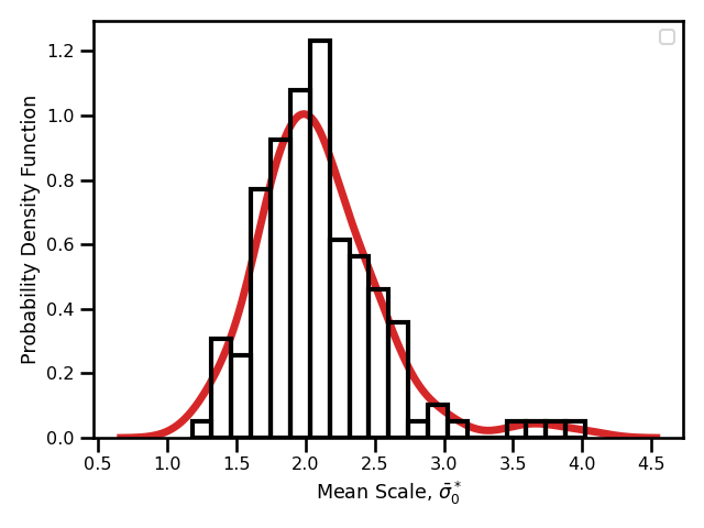 The negative log-likelihood loss (equation
 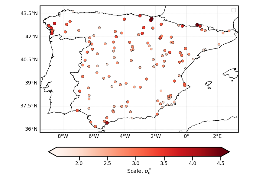 The negative log-likelihood loss (equation
 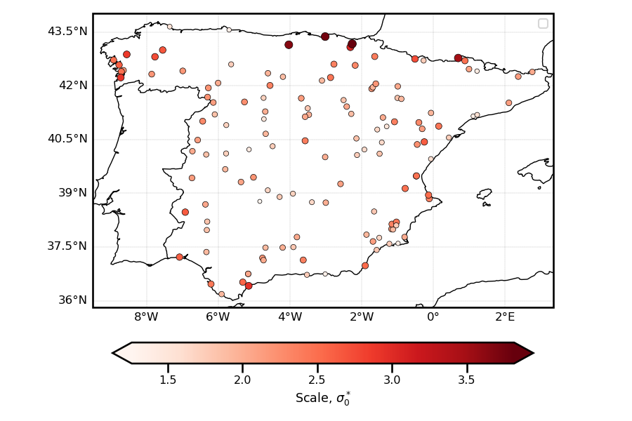 The negative log-likelihood loss (equation
 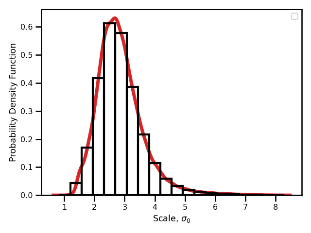 The negative log-likelihood loss (equation
 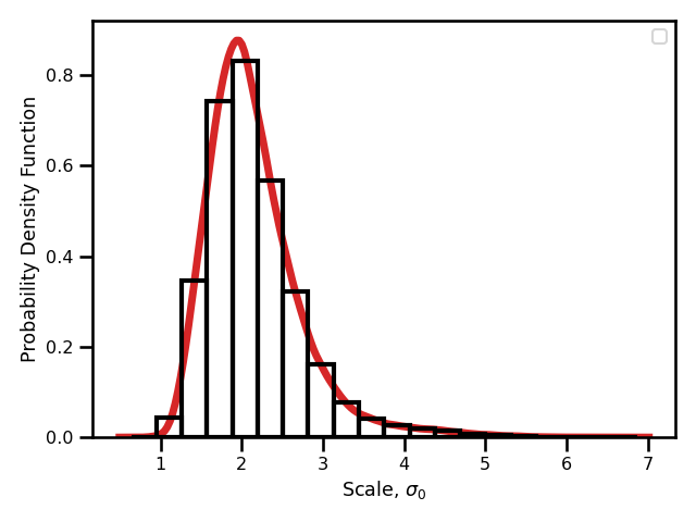 The negative log-likelihood loss (equation
 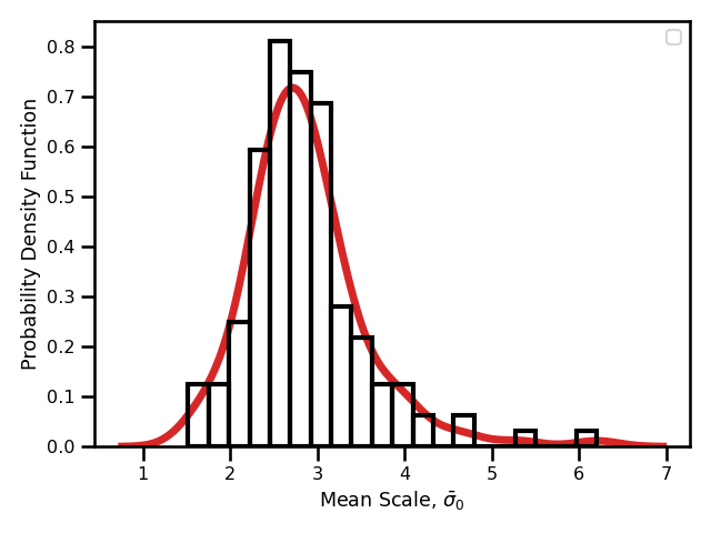 The negative log-likelihood loss (equation
 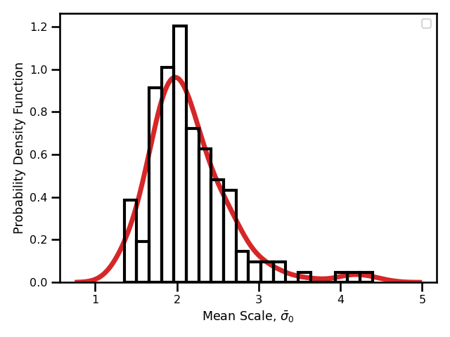 The negative log-likelihood loss (equation
 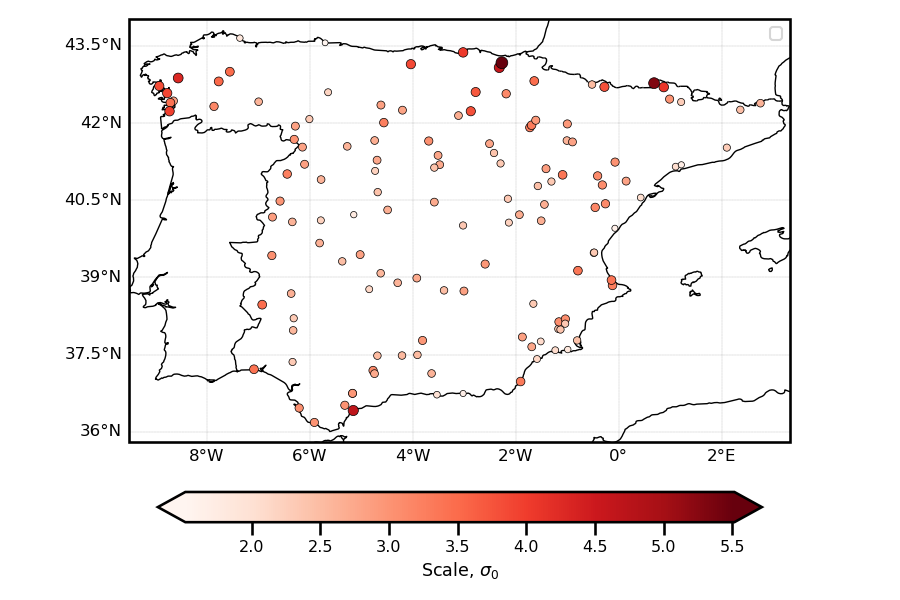 The negative log-likelihood loss (equation
 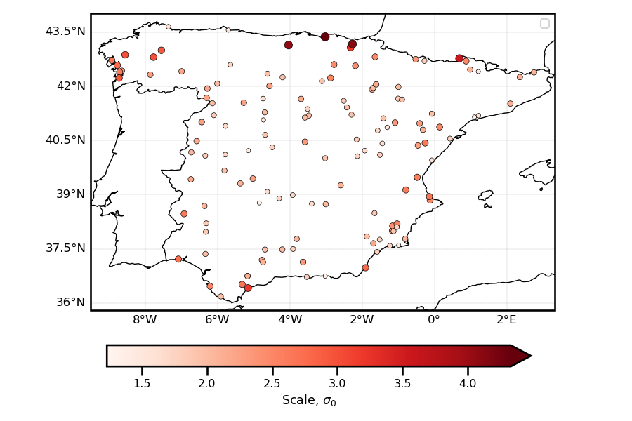 The negative log-likelihood loss (equation
 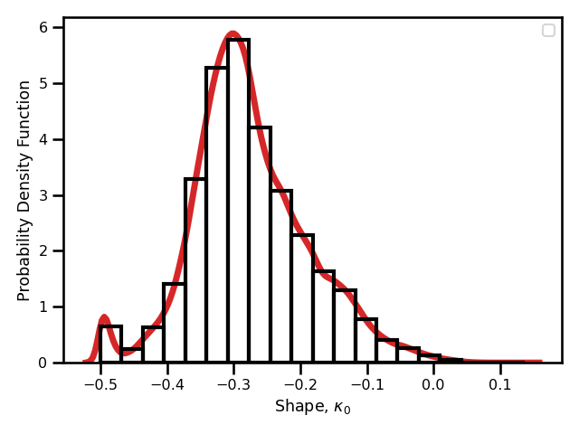 The negative log-likelihood loss (equation
 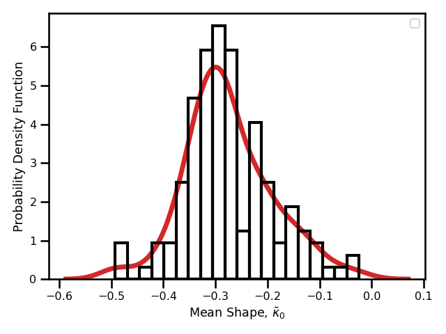 The negative log-likelihood loss (equation
 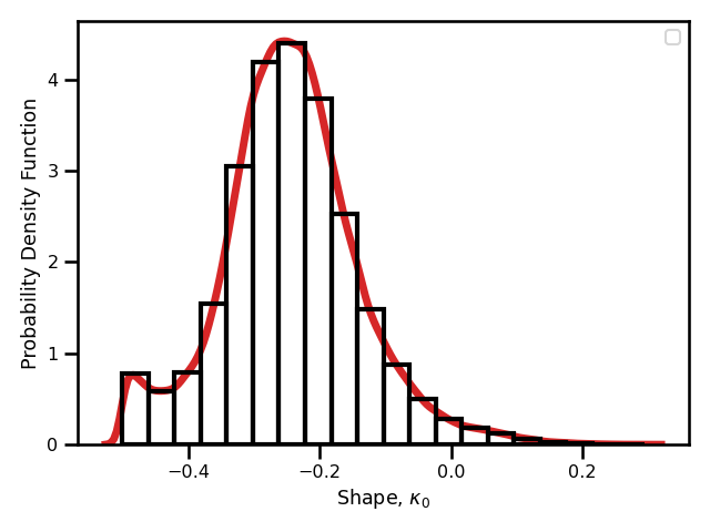 The negative log-likelihood loss (equation
 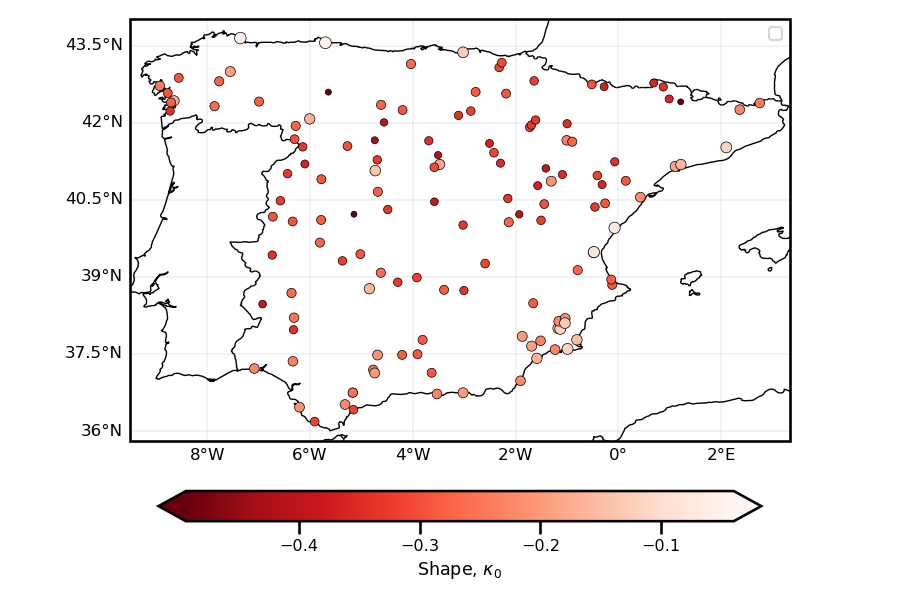 The negative log-likelihood loss (equation
 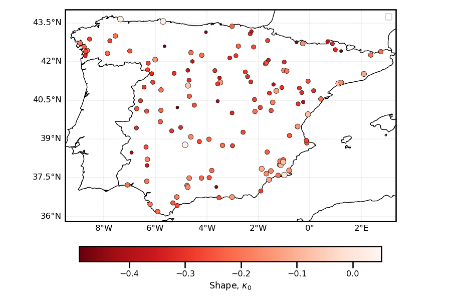 The negative log-likelihood loss (equation
 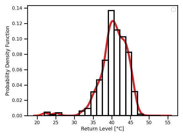 The negative log-likelihood loss (equation (5)) for each time step within the time series.
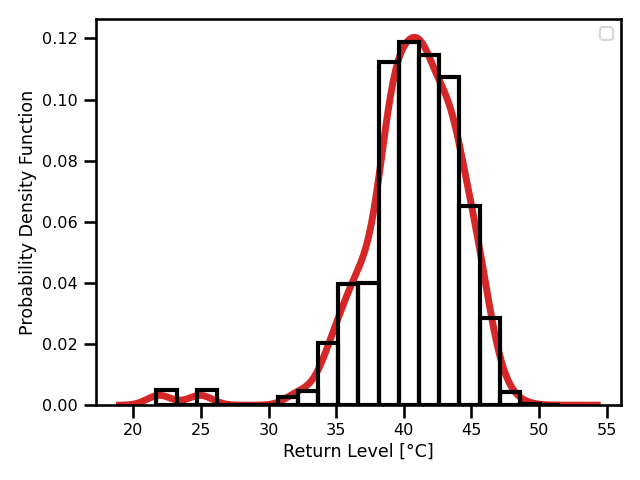 The negative log-likelihood loss (equation (5)) for each time step within the time series.
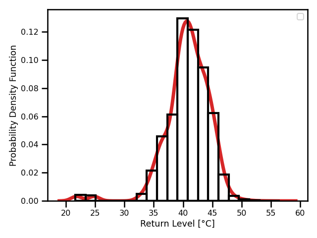 The negative log-likelihood loss (equation
 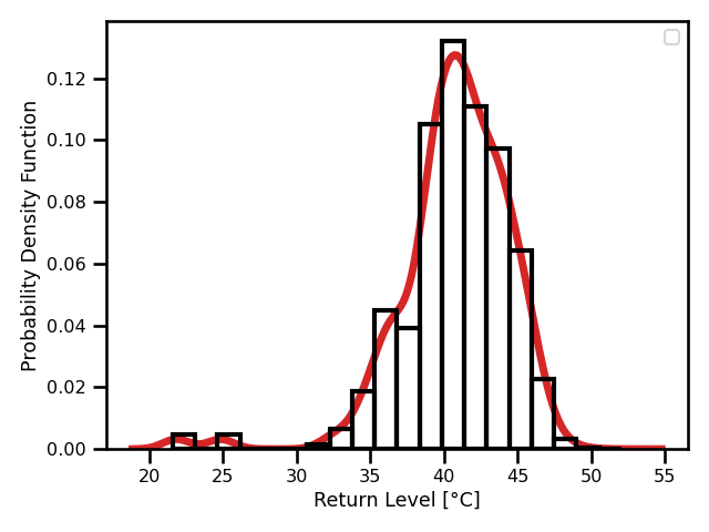 The negative log-likelihood loss (equation
 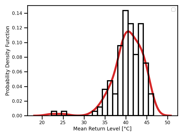 The negative log-likelihood loss (equation (5)) for each time step within the time series.
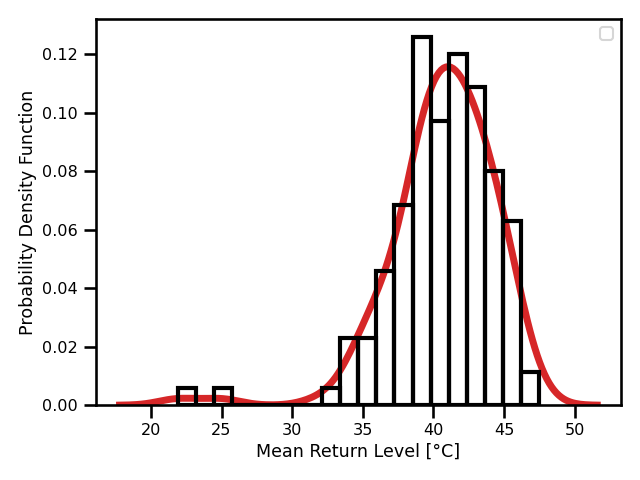 The negative log-likelihood loss (equation (5)) for each time step within the time series.
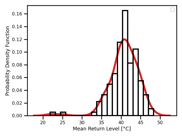 The negative log-likelihood loss (equation
 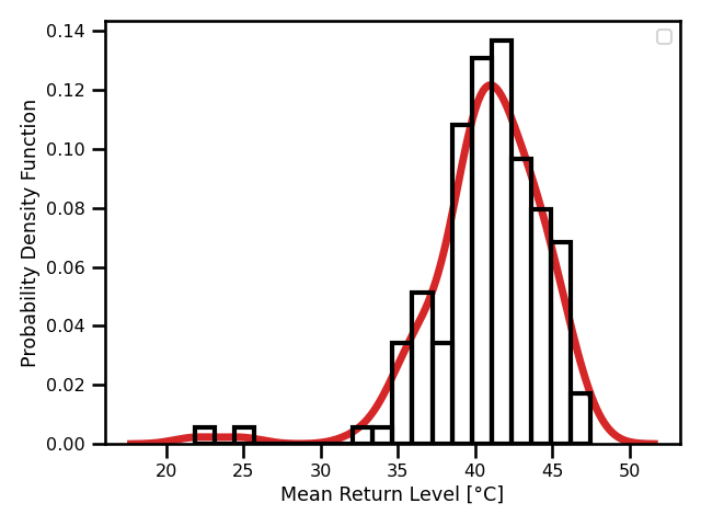 The negative log-likelihood loss (equation
 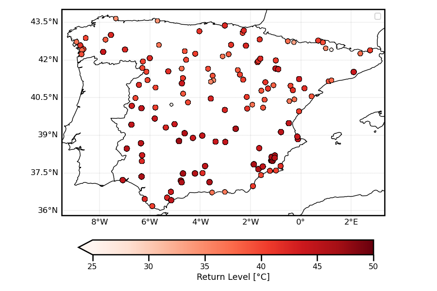 The return period for the iid model.
 The return period for the iid model.
 The return period for the iid model.
 The return period for the iid model.
 The return period for the iid model.