Expectation Propagation from Scratch
This notebook implements expectation propagation (EP) for Gaussian process classification using gaussx primitives. EP approximates non-Gaussian likelihoods with local Gaussian “sites” in natural parameter form, iterating a cavity-update-project loop until convergence.
What you’ll learn:
- The EP algorithm for GP classification with a probit likelihood
- How
GaussianSitesstores per-observation natural parameters - Computing cavity distributions and tilted moments
- Damped site updates via
cvi_update_sites - How sites produce block-diagonal precision via
sites_to_precision
1. Background: EP for GP Classification
In GP classification we place a GP prior over a latent function and connect it to binary labels via a probit likelihood:
where Φ is the standard normal CDF. The posterior is:
This posterior is intractable because the probit factors break conjugacy. EP approximates each likelihood factor with a Gaussian site in natural parameter form:
where is the natural location and encodes the site precision .
The EP loop repeats three steps for each site :
- Cavity: Remove site from the current posterior to get the cavity distribution .
- Tilt: Form the tilted distribution and compute its mean and variance.
- Update: Project the tilted moments back to obtain new site natural parameters, then apply a damped update.
2. Setup and Data Generation
from __future__ import annotations

import warnings


warnings.filterwarnings("ignore", message=r".*IProgress.*")

import jax
import jax.numpy as jnp
import lineax as lx
import matplotlib.pyplot as plt

import gaussx


jax.config.update("jax_enable_x64", True)
Generate 1D binary classification data. The true decision boundary comes from a latent function ; labels are drawn from .
key = jax.random.PRNGKey(42)
N = 30

key, subkey = jax.random.split(key)
X = jnp.sort(jax.random.uniform(subkey, (N,), minval=-3.0, maxval=3.0))

f_true = jnp.sin(2.0 * X)

# Draw binary labels from probit likelihood
key, subkey = jax.random.split(key)
probs = jax.scipy.stats.norm.cdf(f_true)
y = jax.random.bernoulli(subkey, probs).astype(jnp.float64)
y_signed = 2.0 * y - 1.0  # convert to {-1, +1}

fig, ax = plt.subplots(figsize=(10, 4))
ax.scatter(
    X[y == 1],
    y[y == 1],
    s=30,
    c="C0",
    edgecolors="k",
    linewidths=0.5,
    label="y = +1",
    zorder=5,
)
ax.scatter(
    X[y == 0],
    y[y == 0],
    s=30,
    c="C3",
    edgecolors="k",
    linewidths=0.5,
    label="y = -1",
    zorder=5,
)
ax.plot(
    X,
    jax.scipy.stats.norm.cdf(f_true),
    "k--",
    lw=1.5,
    label=r"$\Phi(f^*)$",
    zorder=4,
)
ax.set(xlabel="x", ylabel="y / p(y=1|f*)")
ax.legend(fontsize=9)
ax.set_title("Binary classification data (probit likelihood)")
ax.grid(True, which="major", alpha=0.3)
ax.grid(True, which="minor", alpha=0.1)
ax.minorticks_on()
plt.tight_layout()
plt.show()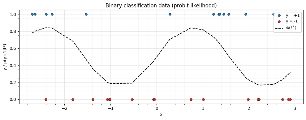
lengthscale = 1.0
variance = 1.0


def rbf_kernel(x1, x2, lengthscale=lengthscale, variance=variance):
    """Squared exponential kernel."""
    sq_dist = (x1[:, None] - x2[None, :]) ** 2
    return variance * jnp.exp(-0.5 * sq_dist / lengthscale**2)


K_prior = rbf_kernel(X, X)
jitter = 1e-6
K_prior = K_prior + jitter * jnp.eye(N)
K_prior_op = lx.MatrixLinearOperator(K_prior)

prior_mean = jnp.zeros(N)
4. Initialize Gaussian Sites
GaussianSites(nat1, nat2) stores per-observation natural parameters.
For scalar EP (), nat1 has shape (N, 1) and nat2 has
shape (N, 1, 1). We initialize both to zero, corresponding to an
uninformative (improper flat) site.
nat1_init = jnp.zeros((N, 1))
nat2_init = jnp.zeros((N, 1, 1))
sites = gaussx.GaussianSites(nat1=nat1_init, nat2=nat2_init)

print(f"Sites nat1 shape: {sites.nat1.shape}")
print(f"Sites nat2 shape: {sites.nat2.shape}")
Sites nat1 shape: (30, 1)
Sites nat2 shape: (30, 1, 1)
5. EP Helper Functions
Tilted moments via Gauss-Hermite quadrature
The tilted distribution for site is:
where is the cavity marginal. We need the mean and variance of .
Using the change of variable with
, we can compute the moments via
Gauss-Hermite quadrature using gaussx.gauss_hermite_points.
gh_points, gh_weights = gaussx.gauss_hermite_points(order=30, dim=1)
gh_z = gh_points[:, 0]  # (P,)

print(f"Gauss-Hermite: {gh_z.shape[0]} quadrature points")


def probit_log_lik(f, y_signed_i):
    """Log probit likelihood: log Phi(y_i * f_i)."""
    return jax.scipy.stats.norm.logcdf(y_signed_i * f)


def tilted_moments(cav_mean_i, cav_var_i, y_signed_i):
    """Compute mean and variance of the tilted distribution via GH quadrature.

    Args:
        cav_mean_i: Cavity mean (scalar).
        cav_var_i: Cavity variance (scalar, positive).
        y_signed_i: Signed label in {-1, +1}.

    Returns:
        (tilt_mean, tilt_var): Mean and variance of tilted distribution.
    """
    cav_std_i = jnp.sqrt(cav_var_i)

    # Transform quadrature points to cavity distribution
    f_pts = cav_mean_i + cav_std_i * gh_z  # (P,)

    # Log-weights: GH weights already account for the Gaussian measure,
    # so we only need the log-likelihood part
    log_lik = jax.vmap(lambda f: probit_log_lik(f, y_signed_i))(f_pts)  # (P,)

    # Normalize in log-space for numerical stability
    log_w = jnp.log(gh_weights) + log_lik
    log_Z = jax.scipy.special.logsumexp(log_w)
    w_normalized = jnp.exp(log_w - log_Z)

    # Tilted moments
    tilt_mean = jnp.sum(w_normalized * f_pts)
    tilt_var = jnp.sum(w_normalized * (f_pts - tilt_mean) ** 2)

    # Clamp variance to stay positive
    tilt_var = jnp.maximum(tilt_var, 1e-10)

    return tilt_mean, tilt_var
Gauss-Hermite: 30 quadrature points
6. The EP Loop
Each EP iteration:
Posterior from prior + sites. The site precision is (diagonal), and the posterior precision is .
Cavity. For each , remove site : , .
Tilted moments. Compute mean and variance of by quadrature.
New site params. Convert tilted moments to natural parameters using
newton_update: the site precision is and .Damped update via
cvi_update_sites.
n_iterations = 15
rho = 0.5  # damping factor
log_z_history = []


def compute_posterior(prior_mean, K_prior_op, sites):
    """Compute the Gaussian posterior from prior + sites."""
    # Site precisions: -2 * nat2, shape (N, 1, 1) -> (N,)
    site_prec = -2.0 * sites.nat2[:, 0, 0]  # (N,)
    site_eta1 = sites.nat1[:, 0]  # (N,)

    # Posterior precision = K^{-1} + diag(site_prec)
    K_inv = gaussx.inv(K_prior_op).as_matrix()
    post_prec_mat = K_inv + jnp.diag(site_prec)
    post_prec_op = lx.MatrixLinearOperator(post_prec_mat)

    # Posterior covariance and mean
    post_cov_mat = gaussx.inv(post_prec_op).as_matrix()
    post_cov_op = lx.MatrixLinearOperator(post_cov_mat)

    # Posterior natural params: eta1_post = K^{-1} mu_prior + site_eta1
    prior_eta1 = gaussx.solve(K_prior_op, prior_mean)
    post_eta1 = prior_eta1 + site_eta1

    post_mean = post_cov_op.mv(post_eta1)

    return post_mean, post_cov_op, post_prec_mat


for iteration in range(n_iterations):
    # Step 1: compute current posterior
    post_mean, post_cov_op, post_prec_mat = compute_posterior(
        prior_mean, K_prior_op, sites
    )
    post_var = jnp.diag(post_cov_op.as_matrix())  # marginal variances

    # Current site params as flat vectors
    site_prec = -2.0 * sites.nat2[:, 0, 0]  # (N,)
    site_eta1 = sites.nat1[:, 0]  # (N,)

    # Step 2-4: for each site, compute cavity -> tilted -> new site
    new_nat1 = jnp.zeros(N)
    new_nat2 = jnp.zeros(N)
    log_z_sum = 0.0

    for i in range(N):
        # Cavity distribution (scalar shortcut)
        cav_prec_i = 1.0 / post_var[i] - site_prec[i]
        cav_prec_i = jnp.maximum(cav_prec_i, 1e-10)
        cav_var_i = 1.0 / cav_prec_i
        cav_mean_i = cav_var_i * (post_mean[i] / post_var[i] - site_eta1[i])

        # Tilted moments
        tilt_mean_i, tilt_var_i = tilted_moments(cav_mean_i, cav_var_i, y_signed[i])

        # New site from moment matching:
        # site_prec_new = 1/tilt_var - 1/cav_var
        # site_eta1_new = tilt_mean/tilt_var - cav_mean/cav_var
        site_prec_new_i = 1.0 / tilt_var_i - cav_prec_i
        site_prec_new_i = jnp.maximum(site_prec_new_i, 1e-10)
        site_eta1_new_i = tilt_mean_i / tilt_var_i - cav_mean_i * cav_prec_i

        new_nat1 = new_nat1.at[i].set(site_eta1_new_i)
        new_nat2 = new_nat2.at[i].set(-0.5 * site_prec_new_i)

        # Log normalizer for convergence monitoring
        z_i = jnp.exp(
            jax.scipy.special.logsumexp(
                jnp.log(gh_weights)
                + jax.vmap(lambda f, yi=y_signed[i]: probit_log_lik(f, yi))(
                    cav_mean_i + jnp.sqrt(cav_var_i) * gh_z
                )
            )
        )
        log_z_sum = log_z_sum + jnp.log(jnp.maximum(z_i, 1e-30))

    # Step 5: damped update via cvi_update_sites
    target_sites = gaussx.GaussianSites(
        nat1=new_nat1[:, None],
        nat2=new_nat2[:, None, None],
    )
    sites = gaussx.cvi_update_sites(sites, target_sites.nat1, target_sites.nat2, rho)

    log_z_history.append(float(log_z_sum))
    print(f"Iteration {iteration + 1:2d}: log Z sum = {log_z_sum:.4f}")
Iteration 1: log Z sum = 6.7737
Iteration 2: log Z sum = 8.3711
Iteration 3: log Z sum = 8.5472
Iteration 4: log Z sum = 8.5733
Iteration 5: log Z sum = 8.5774
Iteration 6: log Z sum = 8.5782
Iteration 7: log Z sum = 8.5787
Iteration 8: log Z sum = 8.5792
Iteration 9: log Z sum = 8.5796
Iteration 10: log Z sum = 8.5800
Iteration 11: log Z sum = 8.5802
Iteration 12: log Z sum = 8.5804
Iteration 13: log Z sum = 8.5805
Iteration 14: log Z sum = 8.5805
Iteration 15: log Z sum = 8.5806
7. Convergence
The sum of log-normalizer terms should stabilize as EP converges.
fig, ax = plt.subplots(figsize=(10, 4))
ax.plot(range(1, n_iterations + 1), log_z_history, "o-", markersize=4)
ax.set(xlabel="EP iteration", ylabel=r"$\sum_i \log Z_i$")
ax.set_title("EP convergence")
ax.grid(True, which="major", alpha=0.3)
ax.grid(True, which="minor", alpha=0.1)
ax.minorticks_on()
plt.tight_layout()
plt.show()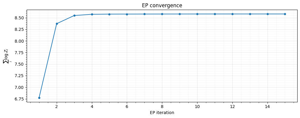
8. Posterior Predictions
Compute the final EP posterior and plot classification probabilities with uncertainty bands.
# Final posterior
post_mean, post_cov_op, post_prec_mat = compute_posterior(prior_mean, K_prior_op, sites)
post_var = jnp.diag(post_cov_op.as_matrix())
post_std = jnp.sqrt(post_var)

# Classification probabilities (integrating out latent f)
# p(y=1|x) = E_q[Phi(f)] = Phi(mu / sqrt(1 + sigma^2))
pred_probs = jax.scipy.stats.norm.cdf(post_mean / jnp.sqrt(1.0 + post_var))

# Confidence bands on latent function
f_upper = post_mean + 2.0 * post_std
f_lower = post_mean - 2.0 * post_std

fig, axes = plt.subplots(2, 1, figsize=(8, 6), sharex=True)

# Top: latent function posterior
ax = axes[0]
ax.fill_between(X, f_lower, f_upper, alpha=0.2, color="C0", label=r"$\mu \pm 2\sigma$")
ax.plot(X, post_mean, "C0-", lw=2, label="EP posterior mean", zorder=3)
ax.plot(X, f_true, "k--", lw=1.5, label="True f(x)", zorder=4)
ax.scatter(
    X[y == 1],
    jnp.ones_like(X[y == 1]) * 1.5,
    c="C0",
    marker="+",
    s=40,
    zorder=5,
)
ax.scatter(
    X[y == 0],
    jnp.ones_like(X[y == 0]) * -1.5,
    c="C3",
    marker="_",
    s=40,
    zorder=5,
)
ax.set(ylabel="f(x)")
ax.legend(fontsize=9)
ax.set_title("EP posterior over latent function")
ax.grid(True, which="major", alpha=0.3)
ax.grid(True, which="minor", alpha=0.1)
ax.minorticks_on()

# Bottom: predictive probabilities
ax = axes[1]
ax.plot(X, pred_probs, "C0-", lw=2, label=r"$p(y=1 \mid x)$", zorder=3)
ax.plot(
    X,
    jax.scipy.stats.norm.cdf(f_true),
    "k--",
    lw=1.5,
    label="True probability",
    zorder=4,
)
ax.scatter(
    X[y == 1],
    y[y == 1],
    s=30,
    c="C0",
    edgecolors="k",
    linewidths=0.5,
    zorder=5,
)
ax.scatter(
    X[y == 0],
    y[y == 0],
    s=30,
    c="C3",
    edgecolors="k",
    linewidths=0.5,
    zorder=5,
)
ax.set(xlabel="x", ylabel="p(y = 1 | x)")
ax.legend(fontsize=9)
ax.set_title("Predictive classification probabilities")
ax.grid(True, which="major", alpha=0.3)
ax.grid(True, which="minor", alpha=0.1)
ax.minorticks_on()

plt.tight_layout()
plt.show()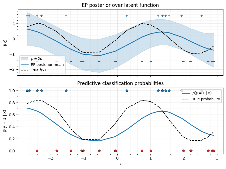
9. Precision Structure via sites_to_precision
The site natural parameters form a diagonal precision contribution.
sites_to_precision wraps these into a BlockTriDiag operator with
zero sub-diagonals --- a block-diagonal structure. In a state-space
GP model, combining this with the prior’s block-tridiagonal precision
yields a full block-tridiagonal posterior precision, enabling
inference.
site_precision = gaussx.sites_to_precision(sites)
print(f"Type: {type(site_precision).__name__}")
print(f"Diagonal blocks shape: {site_precision.diagonal.shape}")
print(f"Sub-diagonal blocks shape: {site_precision.sub_diagonal.shape}")

# Verify sub-diagonals are zero (block-diagonal structure)
print(f"Sub-diagonal norm: {jnp.linalg.norm(site_precision.sub_diagonal):.2e}")
Type: BlockTriDiag
Diagonal blocks shape: (30, 1, 1)
Sub-diagonal blocks shape: (29, 1, 1)
Sub-diagonal norm: 0.00e+00
# Visualize the site precisions (diagonal entries)
site_prec_values = -2.0 * sites.nat2[:, 0, 0]

fig, ax = plt.subplots(figsize=(10, 4))
ax.bar(range(N), site_prec_values, color="C1", alpha=0.7)
ax.set(xlabel="Observation index", ylabel=r"Site precision $\lambda_i$")
ax.set_title("EP site precisions")
ax.set_axisbelow(True)
ax.grid(True, which="major", alpha=0.3)
ax.grid(True, which="minor", alpha=0.1)
ax.minorticks_on()
plt.tight_layout()
plt.show()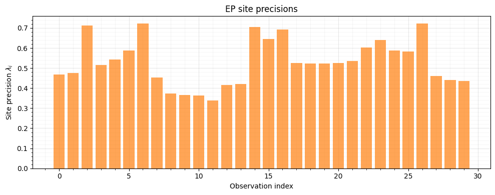
Sites near the decision boundary have higher precision --- EP concentrates its approximation effort where the likelihood is most informative.
10. Using cavity_distribution and newton_update
For completeness, let us verify the gaussx API functions on the final
posterior. cavity_distribution removes a site from the full
posterior, and newton_update converts derivatives into natural
parameters.
# Pick site i = N // 2 (near the middle of the domain)
i = N // 2

# Wrap site i's natural params as lineax operators for cavity_distribution
site_nat1_i = sites.nat1[i, 0]  # scalar
site_nat2_i = -2.0 * sites.nat2[i, 0, 0]  # site precision scalar

# Build full-size vectors/operators for site i
site_nat1_vec = jnp.zeros(N).at[i].set(site_nat1_i)
site_nat2_mat = jnp.diag(jnp.zeros(N).at[i].set(site_nat2_i))
site_nat2_op = lx.MatrixLinearOperator(site_nat2_mat)

cav_mean, cav_cov = gaussx.cavity_distribution(
    post_mean, post_cov_op, site_nat1_vec, site_nat2_op
)

print(f"Cavity mean at i={i}: {cav_mean[i]:.4f}")
print(f"Cavity var  at i={i}: {jnp.diag(cav_cov.as_matrix())[i]:.4f}")
Cavity mean at i=15: 0.3418
Cavity var at i=15: 0.2653
# newton_update: convert Hessian of log-likelihood to site natural params
# For probit, at the posterior mean:
f_i = post_mean[i]
yi = y_signed[i]

# Derivatives of log Phi(y*f) w.r.t. f
pdf_val = jax.scipy.stats.norm.pdf(yi * f_i)
cdf_val = jax.scipy.stats.norm.cdf(yi * f_i)
ratio = pdf_val / jnp.maximum(cdf_val, 1e-10)
jacobian_i = yi * ratio
hessian_i = -(ratio**2 + yi * f_i * ratio)

# newton_update expects arrays
mean_arr = jnp.array([f_i])
jac_arr = jnp.array([jacobian_i])
hess_arr = jnp.array([[hessian_i]])

nat1_newton, nat2_newton = gaussx.newton_update(mean_arr, jac_arr, hess_arr)
print(f"Newton nat1: {nat1_newton[0]:.4f}")
print(f"Newton nat2 (= -hessian): {nat2_newton[0, 0]:.4f}")
Newton nat1: -0.7967
Newton nat2 (= -hessian): 0.6590
Summary
This notebook demonstrated EP for GP classification from scratch using gaussx building blocks:
| gaussx API | Role in EP |
|---|---|
GaussianSites(nat1, nat2) | Store per-site natural parameters |
cvi_update_sites(sites, ...) | Damped natural parameter update |
sites_to_precision(sites) | Convert sites to BlockTriDiag precision |
cavity_distribution(...) | Remove a site from the posterior |
newton_update(mean, jac, hess) | Derivatives to natural parameters |
gauss_hermite_points(order, dim) | Quadrature for tilted moments |
BlockTriDiag | Structured block-tridiagonal operator |
Key takeaways:
- EP iterates cavity-tilt-project to approximate non-Gaussian likelihoods with local Gaussian sites.
- The natural parameterization (, ) makes site addition and removal simple additions in parameter space.
sites_to_precisionproduces aBlockTriDiagthat can be combined with state-space GP priors for scalable temporal inference.- Damping (
rho < 1) incvi_update_sitesis essential for EP stability.