Training a Markov GP — hyperparameter learning

MarkovGPPrior.log_marginal(y, noise_var) is the Kalman-filter marginal likelihood. It is differentiable in every kernel hyperparameter (variance, lengthscale, noise_var, ...) thanks to JAX’s automatic differentiation through the SDE construction and the lax.scan-based filter. That makes hyperparameter learning a one-line gradient descent.

This notebook

generates a noisy 1-D time series,
defines a MaternSDE prior and treats (log_variance, log_lengthscale, log_noise_var) as free parameters,
minimises the negative log marginal likelihood via L-BFGS,
visualises the learned predictive against the data.

import equinox as eqx
import jax
import jax.numpy as jnp
import matplotlib.pyplot as plt
import numpy as np
import optax

from pyrox.gp import MarkovGPPrior, MaternSDE


plt.rcParams["figure.dpi"] = 110
key = jax.random.PRNGKey(0)

/home/azureuser/localfiles/pyrox/.venv/lib/python3.13/site-packages/tqdm/auto.py:21: TqdmWarning: IProgress not found. Please update jupyter and ipywidgets. See https://ipywidgets.readthedocs.io/en/stable/user_install.html
  from .autonotebook import tqdm as notebook_tqdm

Synthetic data¶

A noisy mixture of two sinusoids on an irregular time grid. Wide enough lengthscale that a Matern-3/2 SDE prior fits cleanly.

N = 60
t_clean = jnp.linspace(0.0, 8.0, N)
times = jnp.sort(t_clean + 0.05 * jax.random.normal(jax.random.PRNGKey(2), (N,)))
f_true = 1.2 * jnp.sin(0.9 * times) + 0.4 * jnp.cos(2.7 * times)
y = f_true + 0.18 * jax.random.normal(key, (N,))

fig, ax = plt.subplots(figsize=(8, 3))
ax.scatter(times, y, c="C3", s=14, label="noisy observations")
ax.plot(times, f_true, "k--", lw=1, label="true f")
ax.set_xlabel("t")
ax.set_ylabel("y")
ax.set_title("Noisy time series")
ax.legend(fontsize=8)
plt.tight_layout()
plt.show()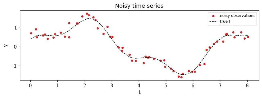

Parameterise the hyperparameters¶

We optimise in log-space so the constraint $\sigma^2, \ell, \sigma_n^2 > 0$ is automatically satisfied. The model lives in a tiny equinox.Module so it composes cleanly with optax.

class MarkovGPModel(eqx.Module):
    log_variance: jax.Array
    log_lengthscale: jax.Array
    log_noise_var: jax.Array
    times: jax.Array

    def __init__(self, times: jax.Array, init: tuple[float, float, float]) -> None:
        self.log_variance = jnp.asarray(jnp.log(init[0]))
        self.log_lengthscale = jnp.asarray(jnp.log(init[1]))
        self.log_noise_var = jnp.asarray(jnp.log(init[2]))
        self.times = times

    def neg_log_marginal(self, y: jax.Array) -> jax.Array:
        sde = MaternSDE(
            variance=jnp.exp(self.log_variance),
            lengthscale=jnp.exp(self.log_lengthscale),
            order=1,
        )
        prior = MarkovGPPrior(sde, self.times)
        return -prior.log_marginal(y, jnp.exp(self.log_noise_var))


model = MarkovGPModel(times, init=(0.5, 0.5, 0.1))
print(f"initial NLL: {float(model.neg_log_marginal(y)):.3f}")

initial NLL: 25.522

Optimise with L-BFGS¶

@eqx.filter_jit
def loss_and_grad(m: MarkovGPModel, y: jax.Array) -> tuple[jax.Array, MarkovGPModel]:
    return eqx.filter_value_and_grad(lambda mm: mm.neg_log_marginal(y))(m)


opt = optax.lbfgs()
params, static = eqx.partition(model, eqx.is_array)
opt_state = opt.init(params)


@eqx.filter_jit
def step(params, static, opt_state, y):
    m = eqx.combine(params, static)
    val, grads = loss_and_grad(m, y)
    grad_params, _ = eqx.partition(grads, eqx.is_array)
    updates, opt_state = opt.update(
        grad_params,
        opt_state,
        params,
        value=val,
        grad=grad_params,
        value_fn=lambda p: eqx.combine(p, static).neg_log_marginal(y),
    )
    params = optax.apply_updates(params, updates)
    return params, opt_state, val


losses = []
hyper_traces = {"variance": [], "lengthscale": [], "noise_var": []}
for it in range(40):
    params, opt_state, val = step(params, static, opt_state, y)
    losses.append(float(val))
    m_now = eqx.combine(params, static)
    hyper_traces["variance"].append(float(jnp.exp(m_now.log_variance)))
    hyper_traces["lengthscale"].append(float(jnp.exp(m_now.log_lengthscale)))
    hyper_traces["noise_var"].append(float(jnp.exp(m_now.log_noise_var)))

trained = eqx.combine(params, static)
print(f"final NLL: {losses[-1]:.3f}")
print(f"learned variance:    {hyper_traces['variance'][-1]:.3f}")
print(f"learned lengthscale: {hyper_traces['lengthscale'][-1]:.3f}")
print(f"learned noise_var:   {hyper_traces['noise_var'][-1]:.4f}")

final NLL: -16.552
learned variance:    0.410
learned lengthscale: 1.692
learned noise_var:   0.0203

Convergence diagnostics¶

fig, axes = plt.subplots(1, 2, figsize=(11, 3.4))
axes[0].plot(losses, "C0", lw=1.5)
axes[0].set_xlabel("iteration")
axes[0].set_ylabel("− log marginal likelihood")
axes[0].set_title("L-BFGS convergence")
axes[0].grid(alpha=0.3)

axes[1].plot(hyper_traces["variance"], label=r"$\sigma^2$", color="C0")
axes[1].plot(hyper_traces["lengthscale"], label=r"$\ell$", color="C2")
axes[1].plot(hyper_traces["noise_var"], label=r"$\sigma_n^2$", color="C3")
axes[1].set_xlabel("iteration")
axes[1].set_ylabel("hyperparameter value")
axes[1].set_title("Hyperparameter trajectories")
axes[1].set_yscale("log")
axes[1].legend(fontsize=9)
axes[1].grid(alpha=0.3)
plt.tight_layout()
plt.show()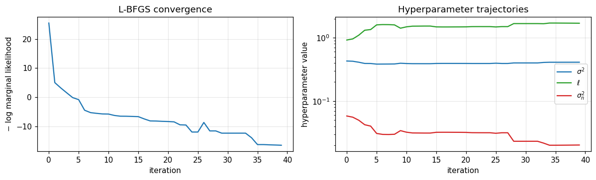

Posterior predictive at the learned hyperparameters¶

sde_final = MaternSDE(
    variance=jnp.exp(trained.log_variance),
    lengthscale=jnp.exp(trained.log_lengthscale),
    order=1,
)
prior_final = MarkovGPPrior(sde_final, times)
cond = prior_final.condition(y, jnp.exp(trained.log_noise_var))

t_star = jnp.linspace(times[0] - 0.3, times[-1] + 1.2, 300)
m_star, v_star = cond.predict(t_star)
m_star, v_star = np.asarray(m_star), np.asarray(v_star)
sd_star = np.sqrt(np.maximum(v_star, 0))

fig, ax = plt.subplots(figsize=(8.5, 3.6))
ax.fill_between(
    t_star,
    m_star - 2 * sd_star,
    m_star + 2 * sd_star,
    color="C0",
    alpha=0.25,
    label="posterior ±2σ",
)
ax.plot(t_star, m_star, color="C0", lw=2, label="posterior mean")
ax.plot(times, f_true, "k--", lw=1, label="true f")
ax.scatter(times, y, c="C3", s=14, label="data", zorder=3)
ax.axvline(times[-1], color="grey", ls=":", lw=0.8, label="end of training")
ax.set_xlabel("t")
ax.set_ylabel("y / f")
ax.set_title("Posterior predictive at learned hyperparameters")
ax.legend(loc="lower left", fontsize=8)
plt.tight_layout()
plt.show()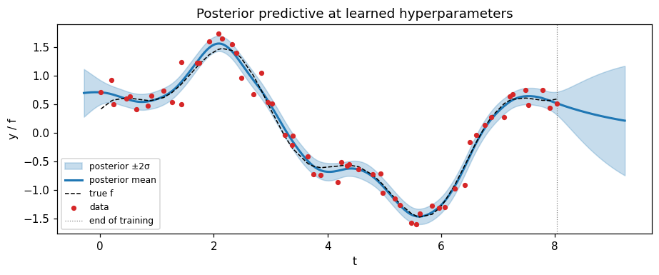

Summary¶

MarkovGPPrior.log_marginal is end-to-end differentiable; any optimiser (L-BFGS, Adam, ...) trains the kernel hyperparameters.
Optimising in log-space sidesteps positivity constraints with no manual reparameterisation gymnastics.
The fitted hyperparameters give a sensible posterior mean and uncertainty band, and the model extrapolates to the prior beyond the training window — the standard stationary-GP behaviour.

For non-Gaussian likelihoods, plug a MarkovGPPrior into one of the strategies in the companion non-Gaussian Markov GP notebook; the same optimisation workflow applies, just with strategy.fit(...).log_marginal_approx as the loss.