Multi-Output Gaussian Processes — LMC, ICM, OILMM

Setup¶

A vector-valued GP $f : \mathbb{R}^d \to \mathbb{R}^P$ assigns to every finite collection of inputs $X = \{x_n\}_{n=1}^N$ a joint Gaussian over $f(X) \in \mathbb{R}^{N \times P}$ . Stacking the columns by $\mathrm{vec}(F)$ — observations of output 1 first, then output 2, etc. — the prior is

\mathrm{vec}(F) \sim \mathcal{N}\!\bigl(0,\, \mathbf{K}\bigr),\qquad \mathbf{K} \in \mathbb{R}^{PN \times PN},

((1))

and the entire question of “what is a multi-output GP” reduces to: what structure does $\mathbf{K}$ have? A plain $PN \times PN$ Gram matrix is too expensive — $\mathcal{O}((PN)^3)$ to factor — and is unstructured: it doesn’t say how outputs are coupled. The three constructions here put successively more structure on $\mathbf{K}$ :

Kernel	Structure imposed on $\mathbf{K}$	Solve cost (Cholesky)	When to use
`LMCKernel`	$\mathbf{K} = \sum_{q=1}^Q B_q \otimes K_q$ with $B_q = w_q w_q^\top$ rank-1	$\mathcal{O}((PN)^3)$ generic; $\mathcal{O}(QN^3)$ when latents tied	Outputs share some structure but each latent has its own kernel / lengthscale.
`ICMKernel`	$\mathbf{K} = B \otimes K$ — a single Kronecker product	$\mathcal{O}(N^3 + P^3)$ via $(B \otimes K)^{-1} = B^{-1} \otimes K^{-1}$	Outputs are smooth versions of one underlying field.
`OILMMKernel`	$\mathbf{K} = \sum_q (w_q w_q^\top) \otimes K_q$ with $W^\top W = I_Q$	$\mathcal{O}(QN^3)$ via projection to $Q$ independent scalar GPs	Many outputs, few latents ( $P \gg Q$ ).

pyrox.gp exposes all three as equinox.Module kernels whose cross_covariance_operator returns a lineax operator carrying the corresponding structure tag (is_kronecker, is_block_diagonal). Downstream gaussx solvers dispatch on those tags so the dense $(PN) \times (PN)$ matrix is never materialised internally.

This notebook walks through:

LMC on two coupled outputs — share information across outputs to predict where one is missing.
ICM as a single-Kronecker special case — show the structure tag pyrox emits so solvers can pick the fast path.
OILMM project / back-project workflow — many outputs, few latents, $Q$ independent scalar GPs.

Setup¶

import subprocess
import sys


try:
    import google.colab  # noqa: F401

    IN_COLAB = True
except ImportError:
    IN_COLAB = False

if IN_COLAB:
    subprocess.run(
        [
            sys.executable,
            "-m",
            "pip",
            "install",
            "-q",
            "pyrox[colab] @ git+https://github.com/jejjohnson/pyrox@main",
        ],
        check=True,
    )

import warnings


warnings.filterwarnings("ignore", message=r".*IProgress.*")

import jax
import jax.numpy as jnp
import jax.random as jr
import matplotlib.pyplot as plt
import numpy as np
from gaussx import is_kronecker

from pyrox.gp import RBF, ICMKernel, LMCKernel, OILMMKernel


jax.config.update("jax_enable_x64", True)

import importlib.util


try:
    from IPython import get_ipython

    ipython = get_ipython()
except ImportError:
    ipython = None

if ipython is not None and importlib.util.find_spec("watermark") is not None:
    ipython.run_line_magic("load_ext", "watermark")
    ipython.run_line_magic(
        "watermark",
        "-v -m -p jax,equinox,gaussx,pyrox,lineax,matplotlib",
    )
else:
    print("watermark extension not installed; skipping reproducibility readout.")

Python implementation: CPython
Python version       : 3.13.5
IPython version      : 9.10.0

jax       : 0.9.2
equinox   : 0.13.6
gaussx    : 0.0.10
pyrox     : 0.0.6
lineax    : 0.1.0
matplotlib: 3.10.8

Compiler    : GCC 11.2.0
OS          : Linux
Release     : 6.8.0-1044-azure
Machine     : x86_64
Processor   : x86_64
CPU cores   : 16
Architecture: 64bit

1. LMC — borrowing strength across outputs¶

Definition¶

The Linear Model of Coregionalization assumes $Q$ independent latent scalar GPs $g_q(x) \sim \mathcal{GP}(0, k_q(x, x'))$ and obtains every output as a linear combination:

f_p(x) = \sum_{q=1}^Q W_{p, q}\, g_q(x), \qquad p = 1, \ldots, P,

((2))

with $W \in \mathbb{R}^{P \times Q}$ a free mixing matrix. The cross-output covariance is, by independence of the $g_q$ ,

\mathrm{Cov}\!\bigl[f_p(x), f_{p'}(x')\bigr] = \sum_{q=1}^Q W_{p, q} W_{p', q}\, k_q(x, x') = \bigl[\textstyle\sum_q B_q\,k_q(x, x')\bigr]_{p, p'},

((3))

where $B_q = w_q w_q^\top \in \mathbb{R}^{P \times P}$ is the rank-1 outer product of the $q$ -th column of $W$ with itself. Stacking observations as $\mathrm{vec}(F) = (F_{:, 1}, F_{:, 2}, \ldots, F_{:, P})$ — output by output — the joint Gram matrix is

\mathbf{K}_{\mathrm{LMC}} = \sum_{q=1}^Q B_q \otimes K_q,\qquad K_q = k_q(X, X) \in \mathbb{R}^{N \times N}.

((4))

The Kronecker structure tells you that LMC adds no new freedom within each latent: $B_q$ is rank-1 by construction. Only the number of latents $Q$ controls expressiveness. When $Q$ different lengthscales are needed (e.g. one fast latent + one slow latent), LMC captures it; when one shared kernel suffices, ICM is the cheaper restriction.

Cross-output reconstruction¶

We hide a chunk of $y_1$ and reconstruct it from $y_2$ via the LMC posterior. Splitting the joint vector into observed indices $\mathcal{O}$ and unobserved $\mathcal{U}$ , the standard Gaussian conditional gives

\mathrm{vec}(F)_\mathcal{U} \mid \mathrm{vec}(Y)_\mathcal{O} \;\sim\; \mathcal{N}\!\Bigl(\mathbf{K}_{\mathcal{U}\mathcal{O}}\,(\mathbf{K}_{\mathcal{O}\mathcal{O}} + \sigma_n^2 I)^{-1}\,\mathrm{vec}(Y)_\mathcal{O},\;\; \mathbf{K}_{\mathcal{U}\mathcal{U}} - \mathbf{K}_{\mathcal{U}\mathcal{O}}\,(\mathbf{K}_{\mathcal{O}\mathcal{O}} + \sigma_n^2 I)^{-1}\,\mathbf{K}_{\mathcal{O}\mathcal{U}}\Bigr).

((5))

An independent per-output GP would have block-diagonal $\mathbf{K}$ , so $\mathbf{K}_{\mathcal{U}\mathcal{O}}$ would be zero between $y_1$ ’s gap entries and $y_2$ ’s observed entries — the conditional mean would collapse to 0 in the gap. LMC’s $\mathbf{K}_{\mathcal{U}\mathcal{O}}$ has off-block entries via $w_{1, q} w_{2, q}\, k_q(x, x')$ , and that’s exactly the route by which $y_2$ informs $y_1$ .

n = 60
key = jr.PRNGKey(0)
key_g1, key_g2, key_eps1, key_eps2 = jr.split(key, 4)
x = jnp.linspace(-3.0, 3.0, n).reshape(-1, 1)

# Two latent GPs with *different* lengthscales — one short, one long. The
# LMC model below uses these same lengthscales, so the data is in-class.
true_kernel_short = RBF(init_variance=1.0, init_lengthscale=0.6)
true_kernel_long = RBF(init_variance=0.5, init_lengthscale=2.0)
K_short = true_kernel_short(x, x) + 1e-8 * jnp.eye(n)
K_long = true_kernel_long(x, x) + 1e-8 * jnp.eye(n)
L_short = jnp.linalg.cholesky(K_short)
L_long = jnp.linalg.cholesky(K_long)
g1 = L_short @ jr.normal(key_g1, (n,))  # short-lengthscale latent
g2 = L_long @ jr.normal(key_g2, (n,))  # long-lengthscale latent

W = jnp.array([[1.0, 0.4], [0.3, 1.1]])
noise_std = 0.05
y1_full = W[0, 0] * g1 + W[0, 1] * g2 + noise_std * jr.normal(key_eps1, (n,))
y2_full = W[1, 0] * g1 + W[1, 1] * g2 + noise_std * jr.normal(key_eps2, (n,))

# Hide the centre of y1 — the LMC must reconstruct it from y2 and the LMC structure.
mask_y1 = (x[:, 0] > -1.0) & (x[:, 0] < 1.0)
y1 = y1_full.at[mask_y1].set(jnp.nan)
y2 = y2_full

Build an LMC kernel with two latent processes and compute the dense $(2N) \times (2N)$ Gram for the joint GP. We do the mask handling by stripping the missing entries from vec(Y); the LMC posterior at those held-out indices is what we want.

# Two latent kernels (give them different lengthscales so LMC ≠ ICM).
lmc = LMCKernel(
    kernels=(
        RBF(pyrox_name="rbf_q0", init_variance=1.0, init_lengthscale=0.6),
        RBF(pyrox_name="rbf_q1", init_variance=0.5, init_lengthscale=2.0),
    ),
    mixing=W,
)

K_full = lmc.full_covariance(x)  # (2N, 2N) — vec ordering: y1 then y2
print(f"LMC Gram shape: {K_full.shape}  (P=2 outputs × N={n} inputs)")

# Build the joint observation vector and apply the missing-entry mask.
# vec(Y) ordering: lmc.full_covariance stacks rows as [output 0 inputs..., output 1 inputs...].
y_vec = jnp.concatenate([y1, y2])
mask_vec = jnp.concatenate([~mask_y1, jnp.ones_like(mask_y1, dtype=bool)])

y_obs = y_vec[mask_vec]
K_oo = K_full[mask_vec][:, mask_vec]  # observed-observed
K_uo = K_full[~mask_vec][:, mask_vec]  # unobserved-observed (the gap entries of y1)
K_uu = K_full[~mask_vec][:, ~mask_vec]

noise_var = noise_std**2
A = K_oo + noise_var * jnp.eye(K_oo.shape[0])
alpha = jnp.linalg.solve(A, y_obs)
mean_gap = K_uo @ alpha
var_gap = jnp.diag(K_uu - K_uo @ jnp.linalg.solve(A, K_uo.T))

LMC Gram shape: (120, 120)  (P=2 outputs × N=60 inputs)

fig, axes = plt.subplots(1, 2, figsize=(18, 5))
# y1 — has the gap.
axes[0].plot(x[:, 0], y1_full, "k--", alpha=0.5, label="true y1")
axes[0].scatter(
    x[~mask_y1, 0],
    y1_full[~mask_y1],
    c="C1",
    edgecolors="k",
    linewidths=0.5,
    zorder=5,
    label="observed y1",
)
axes[0].scatter(
    x[mask_y1, 0],
    mean_gap,
    c="C0",
    edgecolors="k",
    linewidths=0.5,
    zorder=5,
    label="LMC posterior mean (gap)",
)
axes[0].fill_between(
    x[mask_y1, 0],
    mean_gap - 2 * jnp.sqrt(var_gap),
    mean_gap + 2 * jnp.sqrt(var_gap),
    color="C0",
    alpha=0.2,
    label=r"$\pm 2\sigma$",
)
axes[0].axvspan(-1.0, 1.0, color="0.85", alpha=0.4)
axes[0].set_title("y1 — held-out gap reconstructed via LMC + y2")
axes[0].set_xlabel("x")
axes[0].set_ylabel("y1")
axes[0].legend(loc="upper right")

# y2 — fully observed; show LMC sees it.
axes[1].plot(x[:, 0], y2_full, "k--", alpha=0.5, label="true y2")
axes[1].scatter(
    x[:, 0], y2, c="C1", edgecolors="k", linewidths=0.5, zorder=5, label="observed y2"
)
axes[1].axvspan(-1.0, 1.0, color="0.85", alpha=0.4, label="(corresponds to y1's gap)")
axes[1].set_title("y2 — fully observed, drives LMC's gap reconstruction")
axes[1].set_xlabel("x")
axes[1].set_ylabel("y2")
axes[1].legend(loc="upper right")
plt.show()

rmse = float(jnp.sqrt(jnp.mean((mean_gap - y1_full[mask_y1]) ** 2)))
print(f"LMC RMSE on held-out y1 gap: {rmse:.4f}")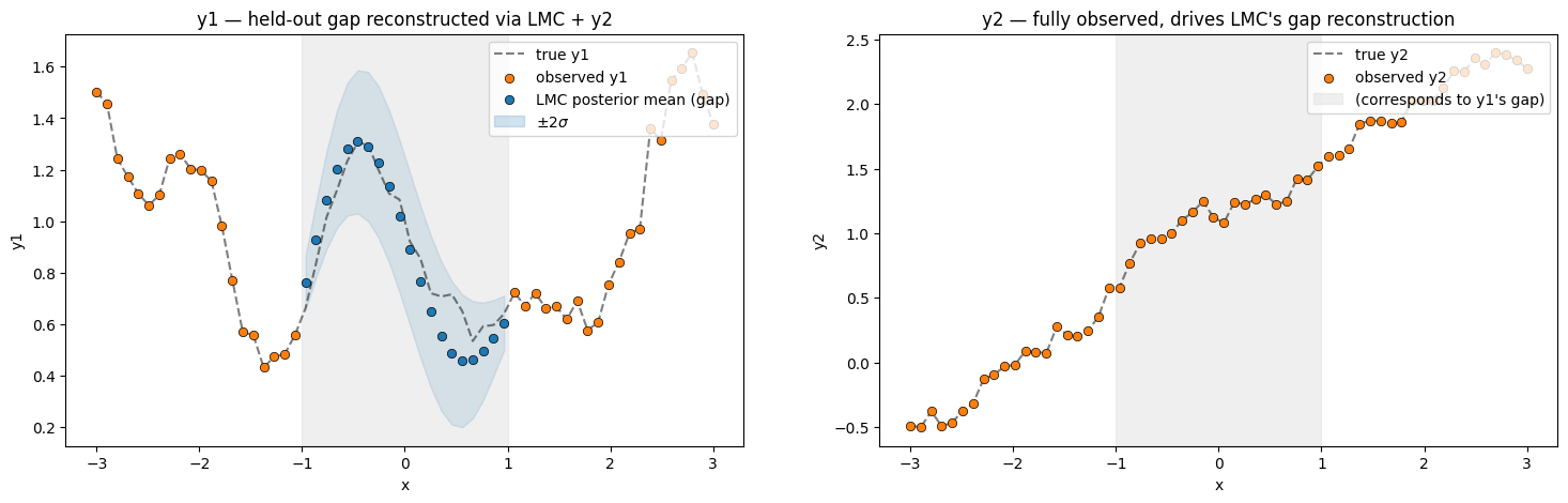

LMC RMSE on held-out y1 gap: 0.0958

The LMC posterior fills the gap in $y_1$ near the truth even though no $y_1$ values were observed in $[-1, 1]$ — the cross-output covariance routes information from $y_2$ through the latent processes back into $y_1$ .

2. ICM — the single-Kronecker special case¶

Definition and derivation¶

The Intrinsic Coregionalization Model is the LMC restriction to a single shared latent kernel: $k_q = k$ for all $q$ . The sum-of-Kroneckers collapses by linearity:

\mathbf{K}_{\mathrm{ICM}} = \sum_{q=1}^Q B_q \otimes K = \Bigl(\sum_q B_q\Bigr) \otimes K = B \otimes K, \qquad B := \sum_q w_q w_q^\top = W W^\top.

((6))

Adding per-output diagonal “nugget” terms $\kappa_p \ge 0$ — extra signal variance unique to each output — gives the standard ICM coregionalization matrix

B = W W^\top + \mathrm{diag}(\kappa) \in \mathbb{R}^{P \times P}.

((7))

Why the Kronecker tag matters¶

Cholesky of a $PN \times PN$ matrix is $\mathcal{O}((PN)^3)$ ; with $P = 3, N = 60$ that is already $\sim 6 \times 10^9$ flops. The Kronecker identity

(B \otimes K)^{-1} = B^{-1} \otimes K^{-1}, \qquad |B \otimes K| = |B|^N\, |K|^P,

((8))

lets gaussx.kronecker_mll evaluate the same log-marginal at $\mathcal{O}(N^3 + P^3)$ — three orders of magnitude cheaper for $N = 60, P = 3$ . The tag is what tells the solver which path to take.

pyrox.gp.ICMKernel.cross_covariance_operator returns a lineax operator with the Kronecker tag set, so any downstream gaussx log-marginal / solve routine can pick the Kronecker-exact path automatically — even though as_matrix() exists for inspection.

icm = ICMKernel(
    kernel=RBF(init_variance=1.0, init_lengthscale=0.6),
    mixing=jnp.array([[1.0, 0.5], [0.5, 1.2], [0.2, 0.9]]),  # P=3 outputs, Q=2 latents
    kappa=jnp.array([0.05, 0.05, 0.05]),  # per-output extra diagonal variance
)

K_op = icm.cross_covariance_operator(x, x)
print(f"ICM operator: {type(K_op).__name__}")
print(f"is_kronecker tag set:    {is_kronecker(K_op)}")
print(f"Operator dense shape:    {K_op.as_matrix().shape}")
print(f"Coregionalization B:\n{icm.coregionalization_matrix()}")

ICM operator: Kronecker
is_kronecker tag set:    True
Operator dense shape:    (180, 180)
Coregionalization B:
[[1.3  1.1  0.65]
 [1.1  1.74 1.18]
 [0.65 1.18 0.9 ]]

is_kronecker(K_op) → True is the load-bearing fact: it tells gaussx that a single Cholesky on the $P \times P$ block factor and a single Cholesky on the $N \times N$ kernel factor are enough — the dense $(PN) \times (PN)$ system is never materialised internally even though as_matrix() exists for inspection.

3. OILMM — project, run scalar GPs, back-project¶

The orthogonality assumption and what it buys¶

OILMM (Bruinsma et al. 2020) is the LMC restricted to a semi-orthogonal mixing matrix:

W \in \mathbb{R}^{P \times Q}, \qquad W^\top W = I_Q, \qquad Q \le P.

((9))

Geometrically, the columns of $W$ are an orthonormal basis of a $Q$ -dimensional subspace of $\mathbb{R}^P$ , and the projector onto that subspace is $WW^\top$ . Within the subspace, $W$ acts isometrically.

Under this constraint, with per-output Gaussian noise $Y_{n, :} = (W g_{n, :}) + \varepsilon_{n, :}$ , $\varepsilon_{n, p} \sim \mathcal{N}(0, \sigma_p^2)$ , the likelihood factorises across latents. Multiplying both sides by $W^\top$ :

\widetilde Y_{n, q} := \bigl(W^\top Y_{n, :}\bigr)_q = g_{n, q} + \widetilde\varepsilon_{n, q}, \qquad \widetilde\varepsilon_{n, q} \sim \mathcal{N}\!\Bigl(0,\, (W^\top \mathrm{diag}(\sigma^2)\, W)_{q, q}\Bigr).

((10))

Critically, the projected noise is diagonal in $q$ when $W$ is orthogonal: there is no off-diagonal coupling between latents after projection (Bruinsma et al. Theorem 1). So the $Q$ projected problems are fully independent: each is a scalar GP regression on $(X, \widetilde Y_{:, q})$ with kernel $k_q$ and noise variance $\widetilde\sigma_q^2 = \sum_p W_{p, q}^2\, \sigma_p^2$ .

The recipe¶

Project observations: $\widetilde Y = Y\, W \in \mathbb{R}^{N \times Q}$ .
Fit $Q$ independent scalar GPs $\widetilde y_{:, q} \mid X \sim \mathcal{GP}(0, k_q) + \widetilde\sigma_q^2 I$ .
Predict in latent space: $\hat g_q(x_*) \sim \mathcal{N}(\hat\mu_q(x_*), \hat\sigma_q^2(x_*))$ .
Back-project to output space:
$\hat Y_{n, p} = \sum_q W_{p, q}\, \hat g_{n, q}, \qquad \mathrm{Var}\!\bigl[\hat Y_{n, p}\bigr] = \sum_q W_{p, q}^2\, \hat\sigma_q^2.$
((11))

Cost. Steps 2-3 are $Q$ scalar GP solves at $\mathcal{O}(QN^3)$ instead of one multi-output solve at $\mathcal{O}((PN)^3)$ . When $P \gg Q$ — many outputs from a few latents — this is a polynomial-degree win. gaussx.oilmm_project and gaussx.oilmm_back_project are the implementation; OILMMKernel.project / back_project are thin wrappers.

P = 4
Q = 2
n_in = 80
key_y, key_w = jr.split(jr.PRNGKey(7), 2)
x_oi = jnp.linspace(-3.0, 3.0, n_in).reshape(-1, 1)

# Generate a random orthogonal mixing matrix via QR.
W_random = jr.normal(key_w, (P, Q))
W_oi, _ = jnp.linalg.qr(W_random)  # (P, Q) with W^T W = I_Q

# Two ground-truth latent GPs (well-separated lengthscales).
true_kernels = [
    RBF(init_variance=1.0, init_lengthscale=0.5),
    RBF(init_variance=0.6, init_lengthscale=2.0),
]
G = jnp.stack(
    [
        jnp.linalg.cholesky(k(x_oi, x_oi) + 1e-8 * jnp.eye(n_in))
        @ jr.normal(jr.fold_in(key_y, q), (n_in,))
        for q, k in enumerate(true_kernels)
    ],
    axis=-1,
)  # (N, Q)

noise_var_per_output = 0.04 * jnp.ones(P)
Y = G @ W_oi.T + jnp.sqrt(noise_var_per_output) * jr.normal(
    jr.fold_in(key_y, 99), (n_in, P)
)

Project the $P$ -dim observations into the $Q$ -dim latent space.

oilmm = OILMMKernel(
    kernels=(
        RBF(pyrox_name="rbf_lat0", init_variance=1.0, init_lengthscale=0.5),
        RBF(pyrox_name="rbf_lat1", init_variance=0.6, init_lengthscale=2.0),
    ),
    mixing=W_oi,
    check_orthogonal=True,
)

Y_lat, noise_lat = oilmm.project(Y, noise_var_per_output)
print(f"Y shape: {Y.shape}")
print(f"Y_latent shape: {Y_lat.shape}  (per-latent observations)")
print(f"per-latent noise variance: {np.asarray(noise_lat)}")

Y shape: (80, 4)
Y_latent shape: (80, 2)  (per-latent observations)
per-latent noise variance: [0.04 0.04]

Now run two independent scalar GP regressions — one per latent — using gaussx.log_marginal_likelihood for each, and do simple posterior-mean prediction in latent space before back-projecting.

def scalar_gp_predict(
    kernel: RBF,
    x_train: jax.Array,
    y_train: jax.Array,
    x_test: jax.Array,
    noise_var: float,
):
    K_xx = kernel(x_train, x_train) + noise_var * jnp.eye(x_train.shape[0])
    K_sx = kernel(x_test, x_train)
    K_ss_diag = kernel.diag(x_test)
    alpha = jnp.linalg.solve(K_xx, y_train)
    mean = K_sx @ alpha
    v = jnp.linalg.solve(K_xx, K_sx.T)
    var = K_ss_diag - jnp.sum(K_sx * v.T, axis=-1)
    return mean, var


x_test = jnp.linspace(-3.5, 3.5, 200).reshape(-1, 1)

f_means = []
f_vars = []
for q, kernel in enumerate(oilmm.independent_gps()):
    mean_q, var_q = scalar_gp_predict(
        kernel, x_oi, Y_lat[:, q], x_test, float(noise_lat[q])
    )
    f_means.append(mean_q)
    f_vars.append(var_q)
F_means = jnp.stack(f_means, axis=-1)  # (M, Q)
F_vars = jnp.stack(f_vars, axis=-1)

# Back-project to the original P=4 output space.
y_means, y_vars = oilmm.back_project(F_means, F_vars)
print(
    f"Back-projected predictive mean shape: {y_means.shape}  (M={x_test.shape[0]}, P={P})"
)

Back-projected predictive mean shape: (200, 4)  (M=200, P=4)

fig, axes = plt.subplots(2, 2, figsize=(18, 9))
for p, ax in enumerate(axes.ravel()):
    ax.scatter(
        x_oi[:, 0],
        Y[:, p],
        c="C1",
        edgecolors="k",
        linewidths=0.5,
        s=20,
        zorder=5,
        label="observed",
    )
    ax.plot(x_test[:, 0], y_means[:, p], color="C0", label="OILMM mean")
    ax.fill_between(
        x_test[:, 0],
        y_means[:, p] - 2 * jnp.sqrt(y_vars[:, p]),
        y_means[:, p] + 2 * jnp.sqrt(y_vars[:, p]),
        color="C0",
        alpha=0.2,
        label=r"$\pm 2\sigma$",
    )
    ax.set_title(f"output {p}")
    ax.set_xlabel("x")
    ax.set_ylabel(f"y_{p}")
    if p == 0:
        ax.legend(loc="upper right")
plt.tight_layout()
plt.show()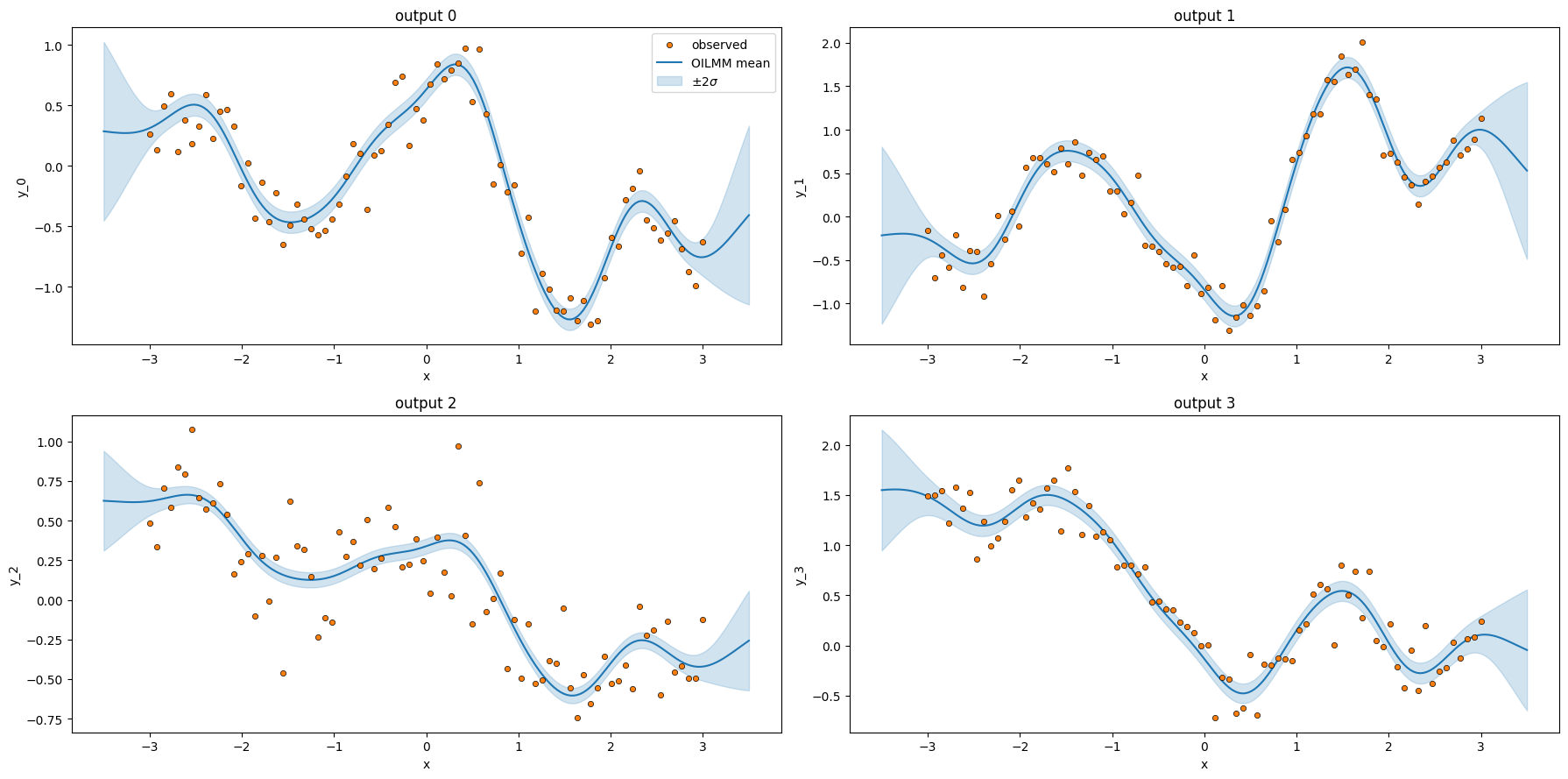

Two scalar GP fits — one per latent — produced predictive means and variances for all four outputs. This is the OILMM win at scale: when $P$ is large but the cross-output structure is low-rank ( $Q \ll P$ ), you pay $Q$ scalar GP costs instead of one monolithic $P$ -output cost.

Sanity check — `oilmm_project` round-trips¶

oilmm_back_project is the inverse of oilmm_project for the orthogonal mixing case. Verify directly:

F_back, _ = oilmm.back_project(Y_lat, jnp.zeros_like(Y_lat))
F_recon = F_back  # back-projected mean
# Project Y_recon → latent and confirm it round-trips.
Y_lat_again, _ = oilmm.project(F_recon, 0.0)
err = float(jnp.max(jnp.abs(Y_lat - Y_lat_again)))
print(f"max round-trip error (project → back-project → project): {err:.2e}")

max round-trip error (project → back-project → project): 1.11e-15

Takeaways¶

LMCKernel: $\mathbf{K} = \sum_q B_q \otimes K_q$ with $B_q = w_q w_q^\top$ rank-1 — the most expressive of the three because every latent has its own kernel $k_q$ . Cross-output coupling enters via the off-block entries of $\mathbf{K}_{\mathcal{U}\mathcal{O}}$ , which is what lets the conditional posterior fill a gap in $y_1$ from observations of $y_2$ .
ICMKernel: the LMC restriction $k_q = k$ , which by linearity collapses to $\mathbf{K} = B \otimes K$ with $B = WW^\top + \mathrm{diag}(\kappa)$ . The is_kronecker tag on the returned lineax operator lets gaussx use $(B \otimes K)^{-1} = B^{-1} \otimes K^{-1}$ for an exact $\mathcal{O}(N^3 + P^3)$ solve instead of $\mathcal{O}((PN)^3)$ .
OILMMKernel: the LMC restriction $W^\top W = I$ , which decouples the projected likelihood ( $\widetilde\varepsilon_q$ are independent across $q$ ) so $\widetilde Y = YW$ becomes $Q$ independent scalar GP problems. Cost drops from $\mathcal{O}((PN)^3)$ to $\mathcal{O}(QN^3)$ — a polynomial win when $P \gg Q$ . Round-trip: project(Y, σ²) → Q scalar GPs → back_project(μ, var).

Multi-Output Gaussian Processes — LMC, ICM, OILMM

Setup¶

Setup¶

1. LMC — borrowing strength across outputs¶

Definition¶

Cross-output reconstruction¶

2. ICM — the single-Kronecker special case¶

Definition and derivation¶

Why the Kronecker tag matters¶

3. OILMM — project, run scalar GPs, back-project¶

The orthogonality assumption and what it buys¶

The recipe¶

Sanity check — oilmm_project round-trips¶

Takeaways¶

Sanity check — `oilmm_project` round-trips¶