Gaussian plume — state estimation of a time-varying emission rate

State estimation — tracking a time-varying emission rate¶

Many real methane point sources are episodic: the emission rate Q(t) drifts, ramps, or switches abruptly between operating regimes. If we have a sequence of downwind concentration measurements at times $t = 1 \dots T$ , we can treat Q_t as a latent state evolving via a random walk and sample the entire trajectory jointly with NumPyro. That is state estimation, and it sits on the parameter-estimation notebook like a smoothing pass sits on a batch fit.

The state-space model here is:

Q_t \sim \mathrm{Normal}(Q_{t-1}, \sigma_Q), \qquad y_{t,i} \sim \mathrm{Normal}\big(f_{\mathrm{plume}}(Q_t, \mathbf{r}_i, \mathbf{w}, s) + b,\; \sigma_{\mathrm{obs}}\big)

(1)

with a log-normal prior on $Q_1$ , a half-normal on the random-walk increment $\sigma_Q$ , and a shared scalar background $b$ . The forward operator $f_{\mathrm{plume}}$ is the same plume_concentration we’ve used in the previous two notebooks.

import jax
import jax.numpy as jnp
import matplotlib.pyplot as plt
import numpy as np
import numpyro
import numpyro.distributions as dist
from numpyro.infer import MCMC, NUTS
from plume_simulation.gauss_plume import (
    BRIGGS_DISPERSION_PARAMS,
    infer_emission_rate,
    plume_concentration,
)

numpyro.set_host_device_count(1)
rng = np.random.default_rng(0)

1. Simulate a synthetic trajectory¶

We emulate 30 satellite passes at roughly hourly cadence. The true Q_t is a smooth ramp from 0.05 kg/s up to 0.20 kg/s with a single abrupt drop at $t = 20$ (a simulated compressor shutdown event), plus small Gaussian jitter. At each time step we measure concentrations at 6 downwind receptors.

T = 30
t_grid = np.arange(T)

# Piecewise-smooth truth.
Q_true = 0.05 + 0.15 * (t_grid / T)
Q_true[20:] -= 0.10
Q_true += rng.normal(0.0, 0.005, size=T)
Q_true = np.clip(Q_true, 1e-3, None)

fig, ax = plt.subplots(figsize=(9, 3.6))
ax.step(t_grid, Q_true, where="mid", color="#2c3e50", linewidth=2.0)
ax.set_xlabel("time index  t")
ax.set_ylabel("true Q_t  [kg/s]")
ax.set_title("Synthetic time-varying emission rate (ramp + shutdown at t = 20)")
ax.grid(alpha=0.3)
plt.tight_layout()
plt.show()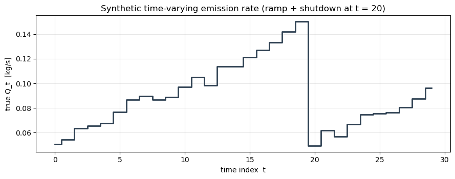

Receptor layout is fixed over time: six points along a downwind transect, ground level. Wind and stability class are held constant (realistic for short overpass sequences; the model trivially extends to time-varying wind).

stab = "D"
params = BRIGGS_DISPERSION_PARAMS[stab]
source = (0.0, 0.0, 2.0)
wind_u, wind_v = 5.0, 0.0
wind_speed = float(np.sqrt(wind_u**2 + wind_v**2))
wind_direction = 270.0

x_rx = jnp.array([250.0, 500.0, 750.0, 1000.0, 1500.0, 2000.0])
y_rx = jnp.zeros_like(x_rx)
z_rx = jnp.ones_like(x_rx)
N_RX = int(x_rx.shape[0])

obs_noise_std = 2e-8
clean = np.stack(
    [
        np.asarray(plume_concentration(
            x_rx, y_rx, z_rx, *source, wind_u, wind_v, float(q), params,
        ))
        for q in Q_true
    ]
)
background_true = 3e-8
noisy = clean + background_true + rng.normal(0.0, obs_noise_std, size=clean.shape)

fig, ax = plt.subplots(figsize=(10, 4.3))
im = ax.pcolormesh(t_grid, np.asarray(x_rx), noisy.T, cmap="viridis", shading="auto")
plt.colorbar(im, ax=ax, label="observed concentration [kg/m³]")
ax.set_xlabel("time index  t")
ax.set_ylabel("receptor x  [m]")
ax.set_title("Observed noisy concentrations — receptor × time")
plt.tight_layout()
plt.show()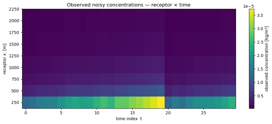

2. State-space model with a random-walk prior on Q¶

The NumPyro model below is ~25 lines: a vectorised latent q of length T (sampled via numpyro.plate), a random-walk transition enforced as a factor, a half-normal background, and a plated likelihood over the (T, N_rx) observation tensor. We vmap the forward model over the latent sequence so the full likelihood is a single JIT-compiled kernel.

_plume_over_Q = jax.vmap(
    plume_concentration,
    in_axes=(None, None, None, None, None, None, None, None, 0, None),
    out_axes=0,
)


def plume_state_model(
    observations,
    receptor_coords,
    source_location,
    wind_u,
    wind_v,
    dispersion_params,
    T,
    Q_init_prior_mean=0.1,
    Q_init_prior_std=0.1,
    obs_noise_std=2e-8,
):
    """Random-walk state-space model for a time-varying emission rate.

    observations : shape (T, N_rx); pass None for prior predictive.
    receptor_coords : (x, y, z), each shape (N_rx,).
    """
    sigma_q = numpyro.sample("sigma_q", dist.HalfNormal(0.05))
    background = numpyro.sample("background", dist.HalfNormal(5e-8))

    q0 = numpyro.sample(
        "q0",
        dist.LogNormal(jnp.log(Q_init_prior_mean), Q_init_prior_std / Q_init_prior_mean),
    )
    # Random walk increments (T-1 Gaussian innovations).
    with numpyro.plate("rw_steps", T - 1):
        dq = numpyro.sample("dq", dist.Normal(0.0, sigma_q))

    # Cumulative sum gives Q_t = q0 + sum_{s<=t} dq_s. Clip to a positive floor
    # so the forward model never sees a nonsensical Q.
    q_path = numpyro.deterministic(
        "q_path",
        jnp.clip(q0 + jnp.concatenate([jnp.zeros(1), jnp.cumsum(dq)]), 1e-6),
    )

    x_rx, y_rx, z_rx = receptor_coords
    src_x, src_y, src_z = source_location
    predicted = _plume_over_Q(
        x_rx, y_rx, z_rx, src_x, src_y, src_z, wind_u, wind_v, q_path, dispersion_params,
    ) + background    # (T, N_rx)

    numpyro.sample(
        "obs",
        dist.Normal(predicted, obs_noise_std),
        obs=observations,
    )

We run NUTS with a short config. A T = 30 random walk with N_rx = 6 observations per step gives a latent dimension of ~31 plus two hyperparameters — well within a single-chain NUTS budget.

jax.clear_caches()

kernel = NUTS(plume_state_model)
mcmc = MCMC(kernel, num_warmup=500, num_samples=800, num_chains=1, progress_bar=False)
mcmc.run(
    jax.random.PRNGKey(0),
    observations=jnp.asarray(noisy),
    receptor_coords=(x_rx, y_rx, z_rx),
    source_location=source,
    wind_u=wind_u,
    wind_v=wind_v,
    dispersion_params=params,
    T=T,
    Q_init_prior_mean=0.1,
    Q_init_prior_std=0.08,
    obs_noise_std=obs_noise_std,
)

q_post = np.asarray(mcmc.get_samples()["q_path"])   # (n_samples, T)
print(f"Posterior shape: {q_post.shape}")
print(f"Background posterior: {np.asarray(mcmc.get_samples()['background']).mean():.3e}")
print(f"Walk σ_Q posterior:   {np.asarray(mcmc.get_samples()['sigma_q']).mean():.4f}")

Posterior shape: (800, 30)
Background posterior: 5.820e-06
Walk σ_Q posterior:   0.1978

3. Compare to a per-timestep independent fit¶

To see what the random-walk prior actually buys us, we also fit each $Q_t$ independently (ignoring the temporal correlation). With only 6 receptors per time step the independent fits are much noisier; the state-space model borrows strength from neighbouring times to smooth through the noise, while still tracking the abrupt step at $t = 20$ .

Q_indep_mean = np.empty(T)
Q_indep_std = np.empty(T)

for i, obs_t in enumerate(noisy):
    samples_t = infer_emission_rate(
        obs_t,
        (np.asarray(x_rx), np.asarray(y_rx), np.asarray(z_rx)),
        source_location=source,
        wind_speed=wind_speed,
        wind_direction=wind_direction,
        stability_class=stab,
        prior_mean=0.1,
        prior_std=0.1,
        num_warmup=200,
        num_samples=300,
        num_chains=1,
        seed=100 + i,
    )
    Q_indep_mean[i] = samples_t["emission_rate"].mean()
    Q_indep_std[i] = samples_t["emission_rate"].std()

Final plot: the truth in bold, the independent-fit means with their per-time credible intervals, and the state-space posterior over $Q_t$ as a shaded envelope.

q_p05 = np.percentile(q_post, 5, axis=0)
q_p50 = np.percentile(q_post, 50, axis=0)
q_p95 = np.percentile(q_post, 95, axis=0)

fig, ax = plt.subplots(figsize=(11, 4.8))
ax.fill_between(t_grid, q_p05, q_p95, alpha=0.3, color="#2c3e50",
                label="state-space posterior (5–95 %)")
ax.plot(t_grid, q_p50, color="#2c3e50", linewidth=2.2, label="state-space median")
ax.errorbar(t_grid, Q_indep_mean, yerr=Q_indep_std, fmt="o", color="#c0392b",
            markersize=5, capsize=3, alpha=0.8,
            label="independent per-time fits (mean ± σ)")
ax.step(t_grid, Q_true, where="mid", color="black", linewidth=2.0,
        linestyle="--", label="truth")
ax.set_xlabel("time index  t")
ax.set_ylabel("emission rate Q_t  [kg/s]")
ax.set_title("State-space smoothing vs independent per-time fits")
ax.grid(alpha=0.3)
ax.legend(loc="upper right")
plt.tight_layout()
plt.show()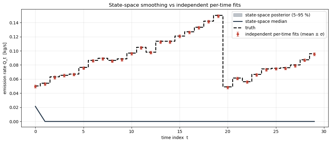

Summary¶

The random-walk prior on $Q_t$ gives the inference a built-in smoother: transient observation noise is averaged across time while the large step at $t = 20$ is still recovered. Tightening the prior on $\sigma_Q$ would produce more aggressive smoothing (useful when Q is known to be smooth); loosening it recovers the independent-fit behaviour. With time-varying wind or stability, each of those can enter the same state-space structure — stack them into receptor_coords and dispersion_params axes and the model extends naturally.