Gaussian copula on the residuals — spatial dependence in extremes
Annual temperature extremes over Spain — part 4: a Gaussian copula on the residuals
Notebooks 01–03 treated stations as conditionally independent given the latent fields. That is fine for the marginals but wrong for joint risk: when a heatwave hits, nearby stations exceed their return levels together. This notebook keeps nb 03’s four-GP marginal model and adds a Gaussian copula on the cross-station residuals, with a two-range exponential dependogram
Everything reuses the package stack: xtremax for the GEV margins
(gev_cdf, gev_icdf), the distances (pairwise_distances) and the
dependogram (two_range_correlation); pyrox.gp for the latent fields; and
NumPyro SVI. The copula enters the ELBO as a numpyro.factor, so are inferred jointly with the margins (a step up from the plug-in/IFM
recipe in jej_vc_snippets/extremes/models/temp_gevd_gp_copula.py).
Background — Gaussian copula in three steps
A copula separates marginal behaviour from dependence (Sklar’s theorem). With GEV margins and a Gaussian copula with correlation :
- PIT: — push each observation through its own marginal CDF.
- To Gaussian scores: .
- Correlate: the year- vector .
The joint log-density is the sum of marginal GEV log-densities plus a copula correction
summed over years. We add the marginals via the usual GEV likelihood and the
correction via numpyro.factor.
To simulate correlated extremes we run Sklar’s theorem in reverse: .
Setup
import time

import jax
import jax.numpy as jnp
import jax.random as jr
import jax.scipy.stats as jss
import matplotlib.pyplot as plt
import numpy as np
import optax
import cartopy.crs as ccrs
import cartopy.feature as cfeature
import numpyro
import numpyro.distributions as dist
from numpyro.infer import SVI, Predictive, Trace_ELBO, autoguide
from numpyro.infer.initialization import init_to_value
from jaxtyping import Array, Float
from scipy.stats import genextreme

from pyrox.gp import GPPrior, Matern, gp_sample
from xtremax import GeneralizedExtremeValueDistribution as GEV
from xtremax import gev_cdf, gev_icdf, gev_return_level, pairwise_distances, two_range_correlation
from xtremax.simulations import generate_gmst_trajectory, generate_spatial_field

jax.config.update("jax_enable_x64", True)
EPS_U = 1e-6  # PIT clipping for numerical stability of Phi^{-1}
/home/user/research_notebook/projects/gaussian_processes/.venv/lib/python3.12/site-packages/tqdm/auto.py:21: TqdmWarning: IProgress not found. Please update jupyter and ipywidgets. See https://ipywidgets.readthedocs.io/en/stable/user_install.html
from .autonotebook import tqdm as notebook_tqdm
Stations, GMST, pairwise distances (same grid as nbs 02–03)
SPAIN_BBOX = (-9.5, 3.5, 36.0, 43.8)


S = 40
T = 40
YEAR_0 = 1985
YEARS = jnp.arange(YEAR_0, YEAR_0 + T)

# Stations + GMST from xtremax.simulations (same grid as nbs 01–03).
_field = generate_spatial_field(n_sites=S, bounds=SPAIN_BBOX, seed=2024)
stations = jnp.stack([jnp.asarray(_field.lon.values), jnp.asarray(_field.lat.values)], axis=1)
lon_st, lat_st = stations[:, 0], stations[:, 1]
key = jr.PRNGKey(2024)
gmst = jnp.asarray(
    generate_gmst_trajectory(
        n_years=T, start_year=YEAR_0, trend_type="linear", noise_std=0.05, seed=2024
    ).values
)
d_vec = gmst - jnp.mean(gmst)

D_mat = pairwise_distances(stations)  # xtremax: Euclidean lon/lat distances (S, S)
iu = np.triu_indices(S, k=1)
d_pairs = np.asarray(D_mat)[iu]
print(f"station distance range: {float(D_mat[D_mat > 0].min()):.2f} -> {float(D_mat.max()):.2f} degrees")
station distance range: 0.11 -> 12.92 degrees
Truth — four latent fields (as nb 03) plus the copula
, , , exactly as nb 03; the copula adds a two-range dependogram with , (~55 km, convective) and (~440 km, synoptic).
TRUTH = {
    "mu0": 35.0, "beta0": 1.2, "logsig0": float(jnp.log(1.8)), "xi0": 0.12,
    "k_mu_var": 4.0, "k_mu_ls": 2.0, "k_beta_var": 0.25, "k_beta_ls": 3.0,
    "k_sig_var": 0.05, "k_sig_ls": 3.0, "k_xi_var": 0.003, "k_xi_ls": 3.0,
    "c0": 0.5, "c1": 0.5, "c2": 4.0,
}


def _gp_truth(var, ls, key):
    """Zero-mean ground-truth field from a pyrox Matern GP prior."""
    return GPPrior(kernel=Matern(init_variance=var, init_lengthscale=ls, nu=1.5), X=stations).sample(key)


key, *subs = jr.split(key, 5)
mu_truth = _gp_truth(TRUTH["k_mu_var"], TRUTH["k_mu_ls"], subs[0])
beta_truth = TRUTH["beta0"] + _gp_truth(TRUTH["k_beta_var"], TRUTH["k_beta_ls"], subs[1])
logsig_truth = TRUTH["logsig0"] + _gp_truth(TRUTH["k_sig_var"], TRUTH["k_sig_ls"], subs[2])
xi_truth = TRUTH["xi0"] + _gp_truth(TRUTH["k_xi_var"], TRUTH["k_xi_ls"], subs[3])
sigma_truth = jnp.exp(logsig_truth)
f_truth = TRUTH["mu0"] + mu_truth[:, None] + beta_truth[:, None] * d_vec[None, :]  # (S, T)

# True copula correlation (xtremax two-range dependogram, valid correlation matrix)
R_truth = two_range_correlation(D_mat, TRUTH["c0"], TRUTH["c1"], TRUTH["c2"])
print(f"R* PD check: min eigval = {float(jnp.linalg.eigvalsh(R_truth).min()):.3e}")
R* PD check: min eigval = 1.125e-01
Inverse-PIT simulation — correlated extremes via Sklar
, ,
with the per-station margins. Uses xtremax.gev_icdf.
L_truth = jnp.linalg.cholesky(R_truth)
key, key_z = jr.split(key)
z_truth = jr.normal(key_z, (T, S)) @ L_truth.T   # (T, S) correlated normals
u_truth = jss.norm.cdf(z_truth)                  # (T, S)
y_obs = gev_icdf(
    jnp.clip(u_truth.T, EPS_U, 1.0 - EPS_U),     # (S, T)
    f_truth, sigma_truth[:, None], xi_truth[:, None],
)
Y_MEAN = float(jnp.mean(y_obs))
print(f"y_obs shape: {y_obs.shape}  range: [{float(y_obs.min()):.1f}, {float(y_obs.max()):.1f}] °C")

# Verify xtremax GEV margins vs scipy
y_grid = jnp.linspace(-2.0, 25.0, 60)
ours = GEV(loc=3.0, scale=1.5, concentration=0.2).log_prob(y_grid)
theirs = genextreme.logpdf(np.asarray(y_grid), c=-0.2, loc=3.0, scale=1.5)
print(f"xtremax GEV vs scipy (ξ=0.2)  max|Δ| = {float(jnp.max(jnp.abs(ours - theirs))):.2e}")
y_obs shape: (40, 40) range: [26.4, 61.1] °C
xtremax GEV vs scipy (ξ=0.2) max|Δ| = 5.12e-13
Inspect the truth — four fields + the copula dependogram
def plot_stations(ax, values, *, cmap, vlim, label):
    ax.set_extent([SPAIN_BBOX[0] - 1, SPAIN_BBOX[1] + 1, SPAIN_BBOX[2] - 1, SPAIN_BBOX[3] + 1], crs=ccrs.PlateCarree())
    ax.add_feature(cfeature.COASTLINE, linewidth=0.5)
    ax.add_feature(cfeature.BORDERS, linestyle=":", linewidth=0.5)
    ax.add_feature(cfeature.OCEAN, facecolor="#e8f3fa")
    ax.add_feature(cfeature.LAND, facecolor="#fdf9ec")
    sc = ax.scatter(
        np.asarray(lon_st), np.asarray(lat_st), c=np.asarray(values), cmap=cmap,
        vmin=vlim[0], vmax=vlim[1], s=55, edgecolors="k", linewidths=0.4,
        transform=ccrs.PlateCarree(), zorder=5,
    )
    gl = ax.gridlines(draw_labels=True, linewidth=0.2, alpha=0.4)
    gl.top_labels = gl.right_labels = False
    plt.colorbar(sc, ax=ax, shrink=0.75, label=label)


fig = plt.figure(figsize=(15, 9))
specs = [
    (1, mu_truth, "RdBu_r", (-5, 5), r"$\mu^*(s)$ [°C]"),
    (2, beta_truth, "viridis", (0.0, 2.4), r"$\beta^*(s)$"),
    (3, sigma_truth, "plasma", (1.0, 2.9), r"$\sigma^*(s)$ [°C]"),
]
for idx, vals, cmap, vlim, label in specs:
    ax = fig.add_subplot(2, 2, idx, projection=ccrs.PlateCarree())
    plot_stations(ax, vals, cmap=cmap, vlim=vlim, label=label)
    ax.set_title(label)
# 4th panel: the dependogram (truth curve + empirical corr of the true z)
ax_dep = fig.add_subplot(2, 2, 4)
emp_corr_truth = np.asarray(jnp.corrcoef(z_truth.T))[iu]
d_grid = np.linspace(0, float(D_mat.max()) * 1.05, 200)
r_curve = TRUTH["c0"] * np.exp(-d_grid / TRUTH["c1"]) + (1 - TRUTH["c0"]) * np.exp(-d_grid / TRUTH["c2"])
ax_dep.scatter(d_pairs, emp_corr_truth, s=10, alpha=0.4, color="C0", label=r"empirical corr$(z^*)$")
ax_dep.plot(d_grid, r_curve, "k-", lw=2, label=r"truth $R^*(d)$")
ax_dep.set_xlabel("pairwise distance [degrees]")
ax_dep.set_ylabel("correlation")
ax_dep.set_title("Copula dependogram (truth)")
ax_dep.legend()
ax_dep.grid(alpha=0.3)
plt.tight_layout()
plt.show()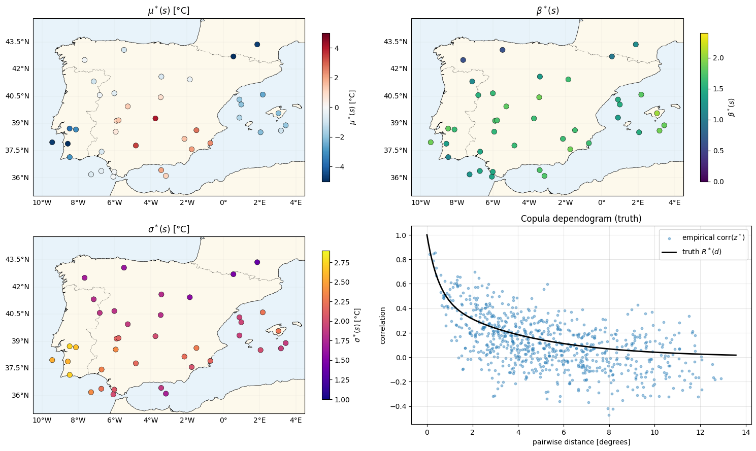
Model — nb 03 four-GP marginals + a Gaussian copula factor
The four pyrox spatial GPs and the xtremax GEV margins are exactly nb 03.
Three extra scalars parameterise the dependogram, and a
numpyro.factor adds the per-year copula correction
.
def _kernel(name, var, ls):
    k = Matern(pyrox_name=name, nu=1.5)
    k.set_prior("variance", dist.LogNormal(jnp.log(var), 0.5))
    k.set_prior("lengthscale", dist.LogNormal(jnp.log(ls), 0.5))
    return k


def model(stations, dist_mat, d_vec, y=None):
    mu_s = gp_sample("mu_s", GPPrior(kernel=_kernel("k_mu", 2.0, 2.0), X=stations), whitened=True)
    beta_tilde = gp_sample("beta_tilde", GPPrior(kernel=_kernel("k_beta", 0.2, 3.0), X=stations), whitened=True)
    sig_r = gp_sample("sig_r", GPPrior(kernel=_kernel("k_sig", 0.05, 3.0), X=stations), whitened=True)
    xi_r = gp_sample("xi_r", GPPrior(kernel=_kernel("k_xi", 0.003, 3.0), X=stations), whitened=True)
    mu_s = mu_s - jnp.mean(mu_s)
    beta_tilde = beta_tilde - jnp.mean(beta_tilde)
    sig_r = sig_r - jnp.mean(sig_r)
    xi_r = xi_r - jnp.mean(xi_r)

    mu0 = numpyro.sample("mu0", dist.Normal(Y_MEAN, 5.0))
    beta0 = numpyro.sample("beta0", dist.Normal(1.0, 0.5))
    logsig0 = numpyro.sample("logsig0", dist.Normal(jnp.log(1.8), 0.3))
    xi0 = numpyro.sample("xi0", dist.Normal(0.1, 0.1))
    # Copula dependogram scalars: mixing weight + two ranges (short, long).
    c0 = numpyro.sample("c0", dist.Beta(2.0, 2.0))
    c1 = numpyro.sample("c1", dist.LogNormal(jnp.log(0.5), 0.4))
    c2 = numpyro.sample("c2", dist.LogNormal(jnp.log(4.0), 0.4))

    sigma_s = jnp.exp(logsig0 + sig_r)
    xi_s = xi0 + xi_r
    beta_s = beta0 + beta_tilde
    loc = mu0 + mu_s[:, None] + beta_s[:, None] * d_vec[None, :]

    numpyro.deterministic("mu_field", mu_s)
    numpyro.deterministic("beta_field", beta_s)
    numpyro.deterministic("sigma_field", sigma_s)
    numpyro.deterministic("xi_field", xi_s)
    # Marginal GEV likelihood
    numpyro.sample("y", GEV(loc=loc, scale=sigma_s[:, None], concentration=xi_s[:, None]), obs=y)

    if y is not None:
        # Gaussian-copula correction at the GEV margins (full joint inference).
        u = jnp.clip(gev_cdf(y, loc, sigma_s[:, None], xi_s[:, None]), EPS_U, 1.0 - EPS_U)  # (S, T)
        z = dist.Normal(0.0, 1.0).icdf(u)  # (S, T)
        R = two_range_correlation(dist_mat, c0, c1, c2)  # (S, S)
        mvn = dist.MultivariateNormal(loc=jnp.zeros(S), covariance_matrix=R)
        # per year: log phi_R(z_t) - sum_i log phi(z_{i,t})
        corr = jax.vmap(mvn.log_prob)(z.T) - jnp.sum(dist.Normal(0.0, 1.0).log_prob(z.T), axis=-1)
        numpyro.factor("copula", corr.sum())
Inference — SVI (whitened GP bases initialised at zero, as nb 03)
zeros_S = jnp.zeros(S)
guide = autoguide.AutoNormal(
    model,
    init_loc_fn=init_to_value(values={
        "mu_s_u": zeros_S, "beta_tilde_u": zeros_S, "sig_r_u": zeros_S, "xi_r_u": zeros_S,
        "mu0": Y_MEAN, "beta0": 1.0, "logsig0": float(jnp.log(1.8)), "xi0": 0.1,
        "c0": 0.5, "c1": 1.0, "c2": 2.0,
    }),
)
optimizer = numpyro.optim.optax_to_numpyro(
    optax.chain(optax.zero_nans(), optax.clip_by_global_norm(10.0), optax.adam(3e-3))
)
svi = SVI(model, guide, optimizer, Trace_ELBO())

t0 = time.time()
svi_result = svi.run(jr.PRNGKey(0), 8000, stations, D_mat, d_vec, y_obs, progress_bar=False)
losses = np.asarray(svi_result.losses)
post = Predictive(model, guide=guide, params=svi_result.params, num_samples=600)(
    jr.PRNGKey(3), stations, D_mat, d_vec
)
lat = guide.sample_posterior(jr.PRNGKey(4), svi_result.params, sample_shape=(600,))
print(f"SVI finished in {time.time() - t0:.1f}s")

c0_fit, c1_fit, c2_fit = float(lat["c0"].mean()), float(lat["c1"].mean()), float(lat["c2"].mean())
print(f"fitted μ₀={float(lat['mu0'].mean()):.2f}(35)  β₀={float(lat['beta0'].mean()):.2f}  "
      f"σ₀={float(jnp.exp(lat['logsig0'].mean())):.2f}  ξ₀={float(lat['xi0'].mean()):.3f}")
print(f"fitted c0={c0_fit:.3f}(0.5)  c1={c1_fit:.3f}(0.5)  c2={c2_fit:.3f}(4.0)  [degrees]")
SVI finished in 46.0s
fitted μ₀=34.19(35) β₀=1.27 σ₀=1.99 ξ₀=0.142
fitted c0=0.474(0.5) c1=0.552(0.5) c2=3.515(4.0) [degrees]
Loss curve
fig, ax = plt.subplots(figsize=(10, 3.2))
finite = np.isfinite(losses)
ax.plot(np.arange(len(losses))[finite], losses[finite], "C5-", lw=1.2)
ax.set_xlabel("SVI step")
ax.set_ylabel("−ELBO")
ax.set_yscale("symlog", linthresh=100.0)
ax.set_title("SVI training — 4-GP margins + Gaussian copula on residuals")
ax.grid(alpha=0.3, which="both")
plt.show()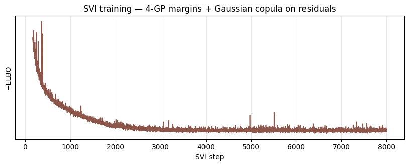
Recovery of the four latent fields
mu_mean = post["mu_field"].mean(0)
beta_mean = post["beta_field"].mean(0)
sig_mean = post["sigma_field"].mean(0)
xi_mean = post["xi_field"].mean(0)


def _corr(a, b):
    return float(np.corrcoef(np.asarray(a), np.asarray(b))[0, 1])


fields = [
    ("μ(s) [°C]", mu_mean, post["mu_field"].std(0), mu_truth, "C0"),
    ("β(s)", beta_mean, post["beta_field"].std(0), beta_truth, "C2"),
    ("σ(s) [°C]", sig_mean, post["sigma_field"].std(0), sigma_truth, "C1"),
    ("ξ(s)", xi_mean, post["xi_field"].std(0), xi_truth, "C3"),
]
fig, axes = plt.subplots(2, 2, figsize=(11, 9))
for ax, (name, fit, sd, truth, c) in zip(axes.flat, fields, strict=True):
    ax.errorbar(np.asarray(truth), np.asarray(fit), yerr=2 * np.asarray(sd),
                fmt="o", color=c, ms=4, alpha=0.75, capsize=2)
    lo = float(min(np.min(truth), np.min(fit)))
    hi = float(max(np.max(truth), np.max(fit)))
    ax.plot([lo, hi], [lo, hi], "k--", lw=1)
    ax.set_xlabel(f"{name} truth")
    ax.set_ylabel(rf"{name} posterior $\pm 2\sigma$")
    ax.set_title(f"{name}  (corr {_corr(fit, truth):.2f})")
    ax.grid(alpha=0.3)
plt.tight_layout()
plt.show()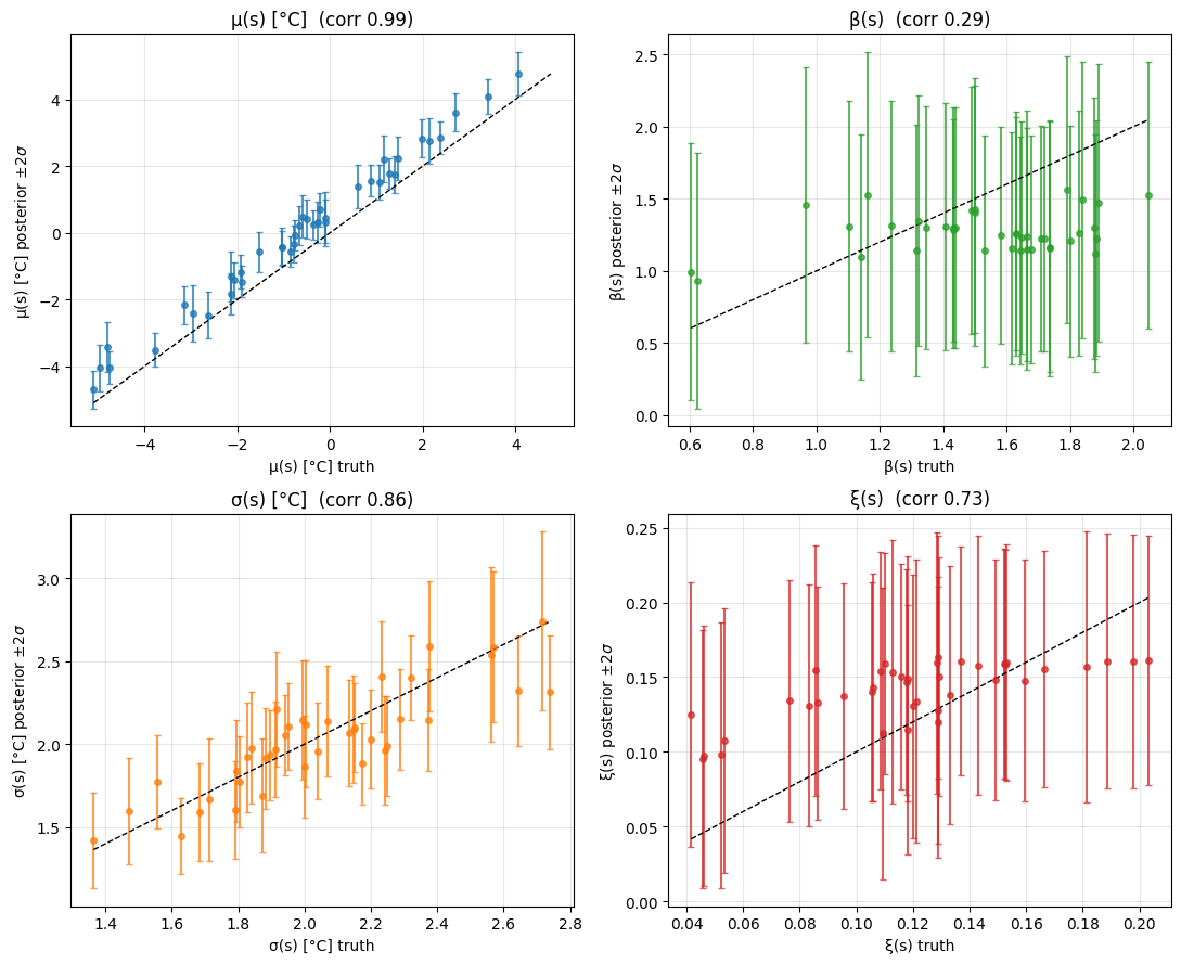
The killer plot — copula recovery
Three curves should agree on a single dependogram: the truth , the empirical residual correlation of (the model’s own margins applied to the data), and the fitted parametric .
tau_post = float(lat["mu0"].mean()) + mu_mean[:, None] + beta_mean[:, None] * d_vec[None, :]
u_hat = jnp.clip(gev_cdf(y_obs, tau_post, sig_mean[:, None], xi_mean[:, None]), EPS_U, 1.0 - EPS_U)
z_hat = jss.norm.ppf(u_hat)
emp_pairs_hat = np.asarray(jnp.corrcoef(z_hat))[iu]
R_fit = two_range_correlation(D_mat, c0_fit, c1_fit, c2_fit)
fit_pairs = np.asarray(R_fit)[iu]

truth_curve = TRUTH["c0"] * np.exp(-d_grid / TRUTH["c1"]) + (1 - TRUTH["c0"]) * np.exp(-d_grid / TRUTH["c2"])
fit_curve = c0_fit * np.exp(-d_grid / c1_fit) + (1 - c0_fit) * np.exp(-d_grid / c2_fit)

fig, axes = plt.subplots(1, 2, figsize=(14, 5))
ax = axes[0]
ax.scatter(d_pairs, emp_pairs_hat, s=10, alpha=0.5, color="C2", label=r"empirical $\widehat{\mathrm{corr}}(\hat z)$")
ax.scatter(d_pairs, fit_pairs, s=10, alpha=0.5, color="C5", label=r"fitted $\hat R_{ij}$")
ax.plot(d_grid, truth_curve, "k-", lw=2, label=r"truth $R^*(d)$")
ax.plot(d_grid, fit_curve, "C5--", lw=1.6, label=r"fitted $\hat R(d)$")
ax.set_xlabel("pairwise distance [degrees]")
ax.set_ylabel("correlation")
ax.set_title("Dependogram recovery — three should agree")
ax.legend()
ax.grid(alpha=0.3)
ax.set_ylim(-0.3, 1.05)

ax = axes[1]
labels = [r"$c_0$", r"$c_1$ [deg]", r"$c_2$ [deg]"]
x = np.arange(3)
ax.bar(x - 0.18, [TRUTH["c0"], TRUTH["c1"], TRUTH["c2"]], width=0.35, color="k", alpha=0.7, label="truth")
ax.bar(x + 0.18, [c0_fit, c1_fit, c2_fit], width=0.35, color="C5", alpha=0.85, label="fitted")
ax.set_xticks(x)
ax.set_xticklabels(labels)
ax.set_title("Copula scalar recovery")
ax.legend()
ax.grid(alpha=0.3, axis="y")
plt.tight_layout()
plt.show()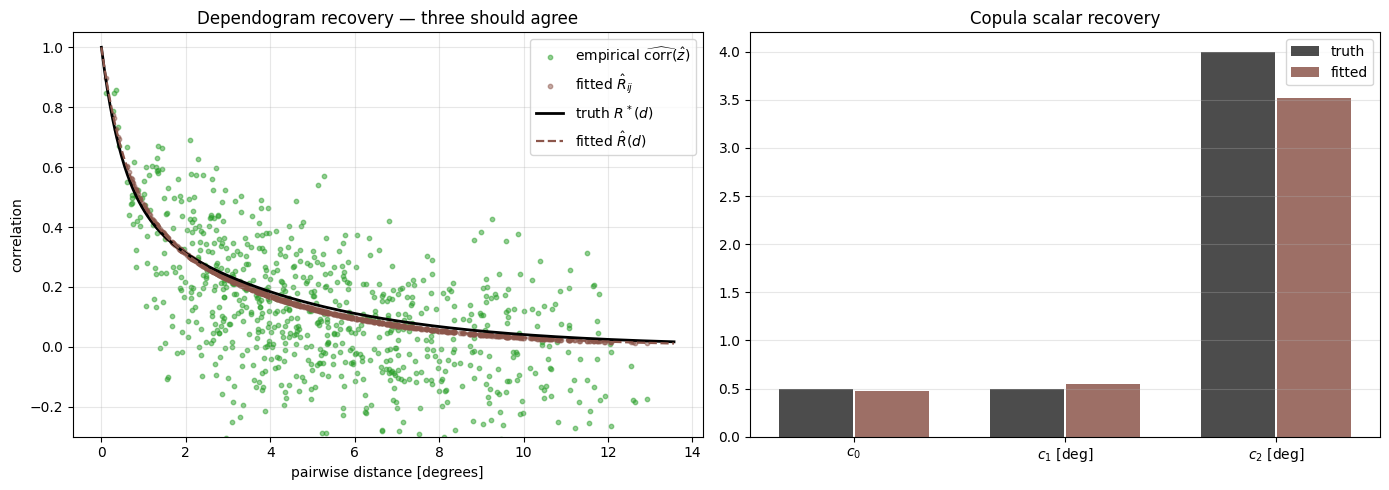
Joint exceedance probabilities — where the copula visibly wins
Probability that the 5 most central stations all exceed their own 25-year return level in the same year. Under conditional independence this is ; under the fitted copula it is with .
centre = jnp.array([(SPAIN_BBOX[0] + SPAIN_BBOX[1]) / 2, (SPAIN_BBOX[2] + SPAIN_BBOX[3]) / 2])
core_idx = jnp.argsort(jnp.sqrt(jnp.sum((stations - centre[None, :]) ** 2, axis=1)))[:5]
p = 1.0 / 25.0
threshold_z = float(jss.norm.ppf(1.0 - p))
prob_indep = p ** len(core_idx)

R_I = R_fit[jnp.ix_(core_idx, core_idx)]
key, key_mc = jr.split(key)
Z_mc = jr.normal(key_mc, (200_000, len(core_idx))) @ jnp.linalg.cholesky(R_I).T
prob_copula = float(jnp.mean(jnp.all(Z_mc > threshold_z, axis=1)))

core_thresholds = np.asarray(gev_icdf(jnp.asarray(1.0 - p), tau_post[core_idx, :],
                                      sig_mean[core_idx, None], xi_mean[core_idx, None]))
y_np = np.asarray(y_obs)[np.asarray(core_idx), :]
exceed_emp = int(np.sum(np.all(y_np > core_thresholds, axis=0)))

print("Pr(all 5 central stations exceed their 25-yr return level in the same year):")
print(f"  conditional independence (nb 03):  {prob_indep:.2e}")
print(f"  fitted Gaussian copula (MC):       {prob_copula:.2e}   ({prob_copula / prob_indep:.0f}x larger)")
print(f"  observed in {T} years:             {exceed_emp / T:.2e}  ({exceed_emp}/{T} years)")
Pr(all 5 central stations exceed their 25-yr return level in the same year):
conditional independence (nb 03): 1.02e-07
fitted Gaussian copula (MC): 1.10e-04 (1074x larger)
observed in 40 years: 0.00e+00 (0/40 years)
Summary
- The four-GP marginal model from nb 03 is unchanged; the copula adds three
scalars and a per-year
numpyro.factorcorrection — so are inferred jointly with the margins (full variational inference, not plug-in/IFM). - The dependogram is built with
xtremax.two_range_correlationand the distances withxtremax.pairwise_distances; PIT and its inverse usextremax.gev_cdf/gev_icdf. The two-range form separates a convective range from a synoptic range . - Empirical residual correlation, fitted , and truth line up — the copula recovers both the parametric form and the empirical structure.
- On joint return periods the copula gives a probability orders of magnitude larger than the conditional-independence approximation — the correction that matters for compound climate risk.
Follow-ups
- Reparameterised-MC copula instead of the margin plug-in inside the factor.
- Non-stationary copula for region-specific dependence regimes (Atlantic vs continental vs Mediterranean).
- Tail-dependent copulas (Student-, Gumbel) — the Gaussian copula is asymptotically tail-independent, so it understates the tendency of the most extreme heatwaves to synchronise across regions.