Non-stationary GEV — location-dependent tails

Annual temperature extremes over Spain — part 3: location-dependent tails¶

Parts 01 and 02 kept the GEV scale σ and shape ξ global — every station shared one tail. This notebook promotes both to per-location spatial GPs, so each site gets its own $\sigma(s)$ and $\xi(s)$ on top of the location $\mu(s)$ and warming rate $\beta(s)$ — four latent spatial fields in total.

Same package stack as before: pyrox.gp whitened gp_sample latents, an xtremax GEV likelihood (now with per-station scale and shape), and NumPyro SVI with an AutoNormal guide.

Background — four-GP latent state¶

\mu(s) \sim \mathcal{GP}(0, k_\mu), \quad \tilde\beta(s) \sim \mathcal{GP}(0, k_\beta), \quad \widetilde{\log\sigma}(s) \sim \mathcal{GP}(0, k_\sigma), \quad \tilde\xi(s) \sim \mathcal{GP}(0, k_\xi),

((1))

combined with scalar intercepts into the per-(s,t) GEV parameters

\mu(s,t) = \mu_0 + \mu(s) + \bigl(\beta_0 + \tilde\beta(s)\bigr) d(t), \quad \sigma(s) = \exp\!\bigl(\log\sigma_0 + \widetilde{\log\sigma}(s)\bigr), \quad \xi(s) = \xi_0 + \tilde\xi(s),

((2))

with $d(t) = \mathrm{GMST}(t) - \overline{\mathrm{GMST}}$ and $y(s,t) \sim \mathrm{GEV}\bigl(\mu(s,t), \sigma(s), \xi(s)\bigr)$ . $\log\sigma$ is modelled (not σ) to keep the scale positive. As before, every latent field is centered so the four scalar intercepts own the global levels.

A caveat up front: ξ is the hardest extreme-value parameter to estimate — 40 years per station carries little information about the tail shape, so the $\xi(s)$ posterior is heavily shrunk toward $\xi_0$ by its GP prior. We recover the pattern of $\xi(s)$ better than its amplitude.

Setup¶

import time

import jax
import jax.numpy as jnp
import jax.random as jr
import matplotlib.pyplot as plt
import numpy as np
import optax
import cartopy.crs as ccrs
import cartopy.feature as cfeature
import numpyro
import numpyro.distributions as dist
from numpyro.infer import SVI, Predictive, Trace_ELBO, autoguide
from numpyro.infer.initialization import init_to_value
from jaxtyping import Array, Float
from scipy.stats import genextreme

from pyrox.gp import GPPrior, Matern, gp_sample
from xtremax import GeneralizedExtremeValueDistribution as GEV
from xtremax import gev_return_level
from xtremax.simulations import generate_gmst_trajectory, generate_spatial_field

jax.config.update("jax_enable_x64", True)

/home/user/research_notebook/projects/gaussian_processes/.venv/lib/python3.12/site-packages/tqdm/auto.py:21: TqdmWarning: IProgress not found. Please update jupyter and ipywidgets. See https://ipywidgets.readthedocs.io/en/stable/user_install.html
  from .autonotebook import tqdm as notebook_tqdm

Data — stations, GMST, and the four truths¶

Stations and GMST are identical to nb 01–02.

SPAIN_BBOX = (-9.5, 3.5, 36.0, 43.8)


S = 40
T = 40
YEAR_0 = 1985
YEARS = jnp.arange(YEAR_0, YEAR_0 + T)

# Stations + GMST from xtremax.simulations (same grid as nbs 01–02).
_field = generate_spatial_field(n_sites=S, bounds=SPAIN_BBOX, seed=2024)
stations = jnp.stack([jnp.asarray(_field.lon.values), jnp.asarray(_field.lat.values)], axis=1)
lon_st, lat_st = stations[:, 0], stations[:, 1]

key = jr.PRNGKey(2024)
gmst = jnp.asarray(
    generate_gmst_trajectory(
        n_years=T, start_year=YEAR_0, trend_type="linear", noise_std=0.05, seed=2024
    ).values
)
d_vec = gmst - jnp.mean(gmst)

Ground-truth latent fields¶

Four independent Matern-3/2 draws. ξ gets a deliberately small variance (0.003) — realistic, since real tail-shape variation is modest.

TRUTH = {
    "mu0": 35.0, "beta0": 1.2, "logsig0": float(jnp.log(1.8)), "xi0": 0.12,
    "k_mu_var": 4.0, "k_mu_ls": 2.0, "k_beta_var": 0.25, "k_beta_ls": 3.0,
    "k_sig_var": 0.05, "k_sig_ls": 3.0, "k_xi_var": 0.003, "k_xi_ls": 3.0,
}


def _gp_truth(var, ls, key):
    """Zero-mean ground-truth field from a pyrox Matern GP prior."""
    return GPPrior(kernel=Matern(init_variance=var, init_lengthscale=ls, nu=1.5), X=stations).sample(key)


key, *subs = jr.split(key, 5)
mu_truth = _gp_truth(TRUTH["k_mu_var"], TRUTH["k_mu_ls"], subs[0])
beta_truth = TRUTH["beta0"] + _gp_truth(TRUTH["k_beta_var"], TRUTH["k_beta_ls"], subs[1])
logsig_truth = TRUTH["logsig0"] + _gp_truth(TRUTH["k_sig_var"], TRUTH["k_sig_ls"], subs[2])
xi_truth = TRUTH["xi0"] + _gp_truth(TRUTH["k_xi_var"], TRUTH["k_xi_ls"], subs[3])
sigma_truth = jnp.exp(logsig_truth)
print(f"mu*(s)    [{float(mu_truth.min()):.2f}, {float(mu_truth.max()):.2f}]")
print(f"beta*(s)  [{float(beta_truth.min()):.2f}, {float(beta_truth.max()):.2f}]")
print(f"sigma*(s) [{float(sigma_truth.min()):.2f}, {float(sigma_truth.max()):.2f}]")
print(f"xi*(s)    [{float(xi_truth.min()):.3f}, {float(xi_truth.max()):.3f}]")

f_truth = TRUTH["mu0"] + mu_truth[:, None] + beta_truth[:, None] * d_vec[None, :]  # (S, T)

mu*(s)    [-5.10, 4.07]
beta*(s)  [0.61, 2.05]
sigma*(s) [1.36, 2.74]
xi*(s)    [0.042, 0.203]

GEV likelihood from `xtremax` (verified vs scipy) + per-station observations¶

Each station draws with its own $(\sigma^*(s), \xi^*(s))$ , broadcast along time.

y_grid = jnp.linspace(-2.0, 25.0, 60)
ours = GEV(loc=3.0, scale=1.5, concentration=0.2).log_prob(y_grid)
theirs = genextreme.logpdf(np.asarray(y_grid), c=-0.2, loc=3.0, scale=1.5)
print(f"xtremax GEV vs scipy (ξ=0.2)  max|Δ| = {float(jnp.max(jnp.abs(ours - theirs))):.2e}")

key, key_obs = jr.split(key)
y_obs = GEV(loc=f_truth, scale=sigma_truth[:, None], concentration=xi_truth[:, None]).sample(key_obs)
Y_MEAN = float(jnp.mean(y_obs))
print(f"y_obs shape: {y_obs.shape}  range: [{float(y_obs.min()):.1f}, {float(y_obs.max()):.1f}] °C")

xtremax GEV vs scipy (ξ=0.2)  max|Δ| = 5.12e-13

y_obs shape: (40, 40)  range: [26.8, 71.9] °C

Four truth maps¶

def plot_stations(ax, values, *, cmap: str, vlim: tuple, label: str) -> None:
    ax.set_extent([SPAIN_BBOX[0] - 1, SPAIN_BBOX[1] + 1, SPAIN_BBOX[2] - 1, SPAIN_BBOX[3] + 1], crs=ccrs.PlateCarree())
    ax.add_feature(cfeature.COASTLINE, linewidth=0.5)
    ax.add_feature(cfeature.BORDERS, linestyle=":", linewidth=0.5)
    ax.add_feature(cfeature.OCEAN, facecolor="#e8f3fa")
    ax.add_feature(cfeature.LAND, facecolor="#fdf9ec")
    sc = ax.scatter(
        np.asarray(lon_st), np.asarray(lat_st), c=np.asarray(values), cmap=cmap,
        vmin=vlim[0], vmax=vlim[1], s=55, edgecolors="k", linewidths=0.4,
        transform=ccrs.PlateCarree(), zorder=5,
    )
    gl = ax.gridlines(draw_labels=True, linewidth=0.2, alpha=0.4)
    gl.top_labels = gl.right_labels = False
    plt.colorbar(sc, ax=ax, shrink=0.75, label=label)


fig = plt.figure(figsize=(14, 9))
specs = [
    (1, mu_truth, "RdBu_r", (-5, 5), r"$\mu^*(s)$ [°C]", r"Spatial offset $\mu^*(s)$"),
    (2, beta_truth, "viridis", (0.0, 2.4), r"$\beta^*(s)$", r"Amplification $\beta^*(s)$"),
    (3, sigma_truth, "plasma", (1.0, 2.9), r"$\sigma^*(s)$ [°C]", r"GEV scale $\sigma^*(s)$"),
    (4, xi_truth, "coolwarm", (0.0, 0.25), r"$\xi^*(s)$", r"GEV shape $\xi^*(s)$"),
]
for idx, vals, cmap, vlim, label, title in specs:
    ax = fig.add_subplot(2, 2, idx, projection=ccrs.PlateCarree())
    plot_stations(ax, vals, cmap=cmap, vlim=vlim, label=label)
    ax.set_title(title)
plt.tight_layout()
plt.show()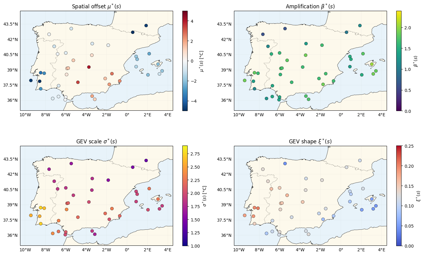

Model — four spatial GPs¶

Four pyrox GPs (distinct pyrox_names), all centered; four scalar intercepts; per-station $\sigma(s)$ and $\xi(s)$ fed straight into the xtremax GEV likelihood.

def _kernel(name, var, ls):
    k = Matern(pyrox_name=name, nu=1.5)
    k.set_prior("variance", dist.LogNormal(jnp.log(var), 0.5))
    k.set_prior("lengthscale", dist.LogNormal(jnp.log(ls), 0.5))
    return k


def model(stations, d_vec, y=None):
    mu_s = gp_sample("mu_s", GPPrior(kernel=_kernel("k_mu", 2.0, 2.0), X=stations), whitened=True)
    beta_tilde = gp_sample("beta_tilde", GPPrior(kernel=_kernel("k_beta", 0.2, 3.0), X=stations), whitened=True)
    sig_r = gp_sample("sig_r", GPPrior(kernel=_kernel("k_sig", 0.05, 3.0), X=stations), whitened=True)
    xi_r = gp_sample("xi_r", GPPrior(kernel=_kernel("k_xi", 0.003, 3.0), X=stations), whitened=True)
    mu_s = mu_s - jnp.mean(mu_s)
    beta_tilde = beta_tilde - jnp.mean(beta_tilde)
    sig_r = sig_r - jnp.mean(sig_r)
    xi_r = xi_r - jnp.mean(xi_r)

    mu0 = numpyro.sample("mu0", dist.Normal(Y_MEAN, 5.0))
    beta0 = numpyro.sample("beta0", dist.Normal(1.0, 0.5))
    logsig0 = numpyro.sample("logsig0", dist.Normal(jnp.log(1.8), 0.3))
    xi0 = numpyro.sample("xi0", dist.Normal(0.1, 0.1))

    beta_s = beta0 + beta_tilde
    sigma_s = jnp.exp(logsig0 + sig_r)  # (S,)
    xi_s = xi0 + xi_r                   # (S,)
    loc = mu0 + mu_s[:, None] + beta_s[:, None] * d_vec[None, :]  # (S, T)

    numpyro.deterministic("mu_field", mu_s)
    numpyro.deterministic("beta_field", beta_s)
    numpyro.deterministic("sigma_field", sigma_s)
    numpyro.deterministic("xi_field", xi_s)
    numpyro.sample("y", GEV(loc=loc, scale=sigma_s[:, None], concentration=xi_s[:, None]), obs=y)

Inference — SVI¶

With four per-station fields, a random whitened-latent start can push some stations’ $\sigma(s)/\xi(s)$ out of GEV support, so we additionally initialise the whitened GP bases (*_u) at zero — at init every station has $\sigma=1.8,\ \xi=0.1$ uniform, comfortably in-support.

zeros_S = jnp.zeros(S)
guide = autoguide.AutoNormal(
    model,
    init_loc_fn=init_to_value(values={
        "mu_s_u": zeros_S, "beta_tilde_u": zeros_S, "sig_r_u": zeros_S, "xi_r_u": zeros_S,
        "mu0": Y_MEAN, "beta0": 1.0, "logsig0": float(jnp.log(1.8)), "xi0": 0.1,
    }),
)
optimizer = numpyro.optim.optax_to_numpyro(
    optax.chain(optax.zero_nans(), optax.clip_by_global_norm(10.0), optax.adam(3e-3))
)
svi = SVI(model, guide, optimizer, Trace_ELBO())

t0 = time.time()
svi_result = svi.run(jr.PRNGKey(0), 8000, stations, d_vec, y_obs, progress_bar=False)
losses = np.asarray(svi_result.losses)
post = Predictive(model, guide=guide, params=svi_result.params, num_samples=600)(
    jr.PRNGKey(3), stations, d_vec
)
lat = guide.sample_posterior(jr.PRNGKey(4), svi_result.params, sample_shape=(600,))
print(f"SVI finished in {time.time() - t0:.1f}s")


def _corr(a, b):
    return float(np.corrcoef(np.asarray(a), np.asarray(b))[0, 1])


sig_fit = post["sigma_field"].mean(0)
xi_fit = post["xi_field"].mean(0)
print(f"fitted μ₀ = {float(lat['mu0'].mean()):.2f} (35)   β₀ = {float(lat['beta0'].mean()):.2f} "
      f"(mean β* {float(beta_truth.mean()):.2f})")
print(f"fitted σ₀ = {float(jnp.exp(lat['logsig0'].mean())):.2f} (mean σ* {float(sigma_truth.mean()):.2f})   "
      f"ξ₀ = {float(lat['xi0'].mean()):.3f} (mean ξ* {float(xi_truth.mean()):.3f})")
print(f"truth-vs-fit corr:  μ={_corr(post['mu_field'].mean(0), mu_truth):.2f}  "
      f"β={_corr(post['beta_field'].mean(0), beta_truth):.2f}  "
      f"σ={_corr(sig_fit, sigma_truth):.2f}  ξ={_corr(xi_fit, xi_truth):.2f}")

SVI finished in 25.2s
fitted μ₀ = 34.33 (35)   β₀ = 1.20 (mean β* 1.53)
fitted σ₀ = 2.06 (mean σ* 2.05)   ξ₀ = 0.152 (mean ξ* 0.120)
truth-vs-fit corr:  μ=0.99  β=0.43  σ=0.87  ξ=0.59

Loss curve¶

fig, ax = plt.subplots(figsize=(10, 3.2))
finite = np.isfinite(losses)
ax.plot(np.arange(len(losses))[finite], losses[finite], "C4-", lw=1.2)
ax.set_xlabel("SVI step")
ax.set_ylabel("−ELBO")
ax.set_yscale("symlog", linthresh=100.0)
ax.set_title("SVI training — four-GP non-stationary GEV")
ax.grid(alpha=0.3, which="both")
plt.show()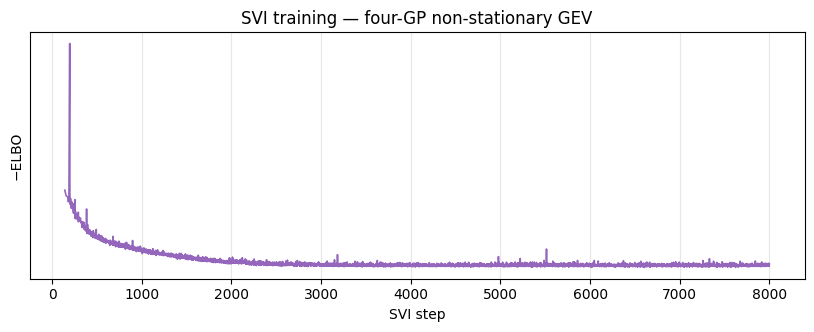

Parameter recovery — four fields¶

Truth-vs-posterior scatter for each latent field. μ and σ recover well; β is shrunk modestly; ξ is the hardest — its posterior is pulled strongly toward $\xi_0$ by the GP prior, so the cloud is compressed along the vertical axis (low amplitude, but the pattern correlation is positive).

fields = [
    ("μ(s) [°C]", post["mu_field"].mean(0), post["mu_field"].std(0), mu_truth, "C0"),
    ("β(s)", post["beta_field"].mean(0), post["beta_field"].std(0), beta_truth, "C2"),
    ("σ(s) [°C]", sig_fit, post["sigma_field"].std(0), sigma_truth, "C1"),
    ("ξ(s)", xi_fit, post["xi_field"].std(0), xi_truth, "C3"),
]
fig, axes = plt.subplots(2, 2, figsize=(11, 9))
for ax, (name, fit, sd, truth, c) in zip(axes.flat, fields, strict=True):
    ax.errorbar(np.asarray(truth), np.asarray(fit), yerr=2 * np.asarray(sd),
                fmt="o", color=c, ms=4, alpha=0.75, capsize=2)
    lo = float(min(np.min(truth), np.min(fit)))
    hi = float(max(np.max(truth), np.max(fit)))
    ax.plot([lo, hi], [lo, hi], "k--", lw=1)
    ax.set_xlabel(f"{name} truth")
    ax.set_ylabel(rf"{name} posterior $\pm 2\sigma$")
    ax.set_title(f"{name}  (corr {_corr(fit, truth):.2f})")
    ax.grid(alpha=0.3)
plt.tight_layout()
plt.show()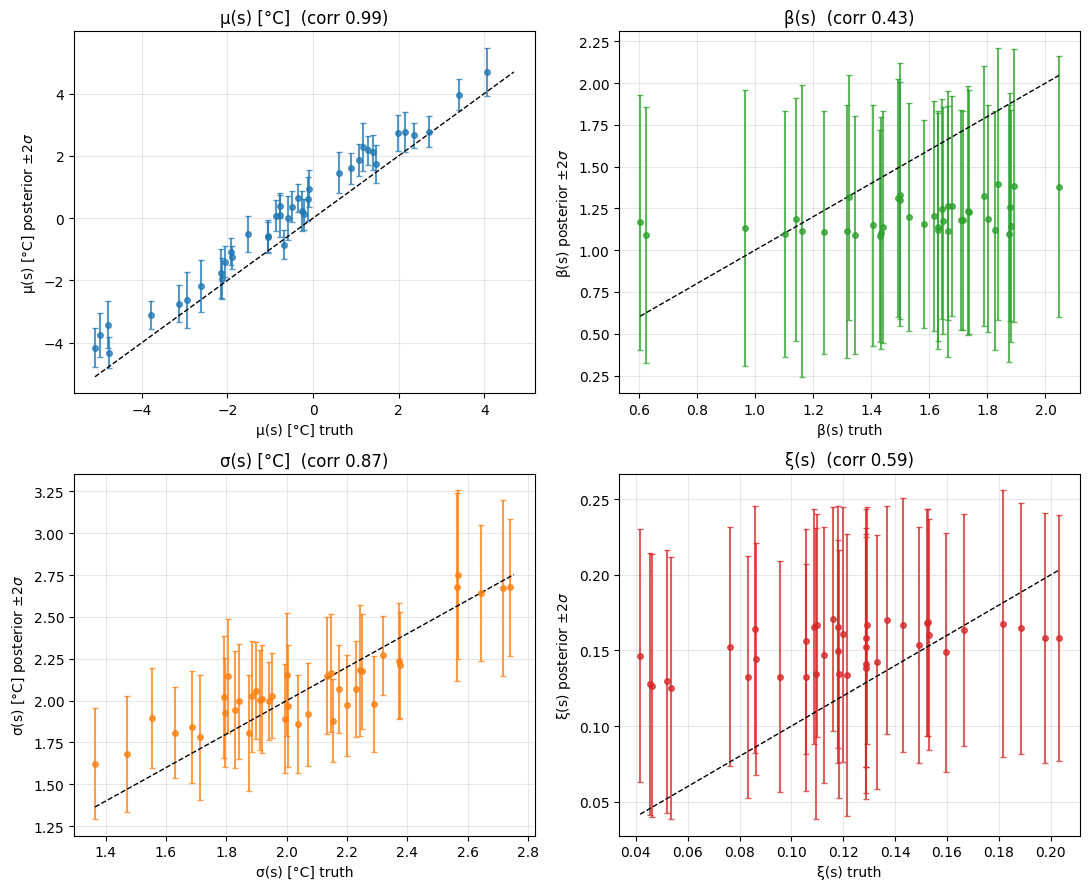

The two spatial signatures — $\hat\sigma(s)$ and $\hat\xi(s)$ ¶

The new ingredients of this notebook: maps of the recovered GEV scale and shape fields, side by side with their truths.

fig = plt.figure(figsize=(14, 9))
sig_specs = [
    (1, sigma_truth, "plasma", (1.0, 2.9), r"$\sigma^*(s)$ — truth"),
    (2, sig_fit, "plasma", (1.0, 2.9), r"$\hat\sigma(s)$ — posterior"),
    (3, xi_truth, "coolwarm", (0.0, 0.25), r"$\xi^*(s)$ — truth"),
    (4, xi_fit, "coolwarm", (0.0, 0.25), r"$\hat\xi(s)$ — posterior"),
]
for idx, vals, cmap, vlim, title in sig_specs:
    ax = fig.add_subplot(2, 2, idx, projection=ccrs.PlateCarree())
    plot_stations(ax, vals, cmap=cmap, vlim=vlim, label=title.split(" ")[0])
    ax.set_title(title)
plt.tight_layout()
plt.show()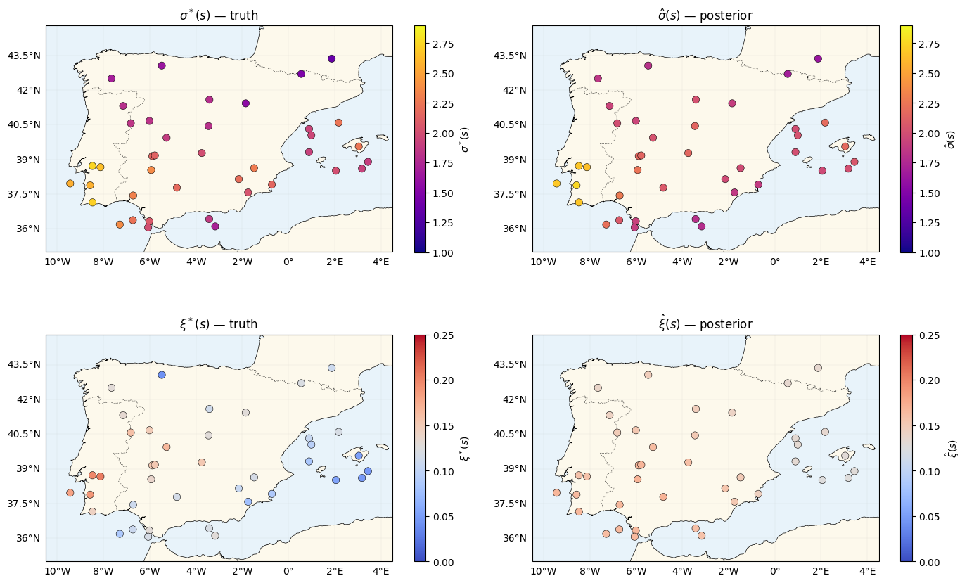

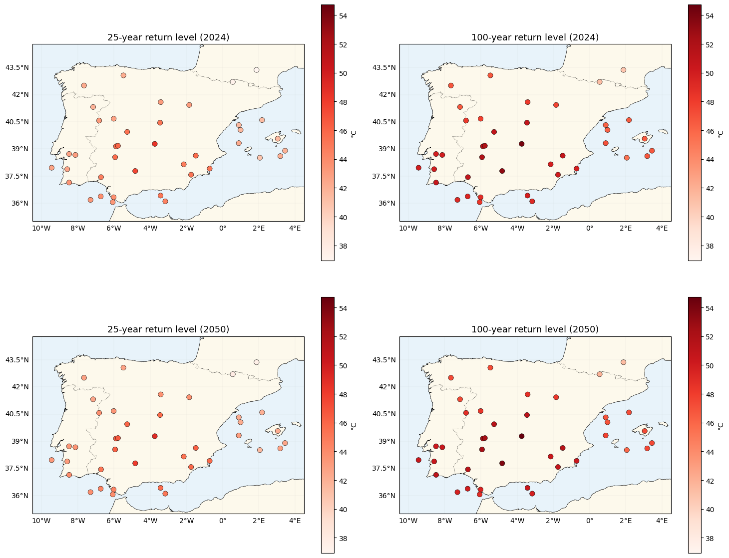
Return-level maps with location-dependent tails¶

Now both the location $\hat\tau(s, t^*)$ and the tail $(\hat\sigma(s), \hat\xi(s))$ vary in space, so the return-level maps carry spatial structure from all four fields. We use xtremax.gev_return_level with per-station scale and shape.

mu0_p = float(lat["mu0"].mean())
mu_field_mean = post["mu_field"].mean(0)
beta_field_mean = post["beta_field"].mean(0)

gmst_2024 = gmst[-1]
gmst_2050 = gmst[-1] + (gmst[-1] - gmst[0]) / (T - 1) * (2050 - (YEAR_0 + T - 1))
tau_2024 = mu0_p + mu_field_mean + beta_field_mean * (gmst_2024 - jnp.mean(gmst))
tau_2050 = mu0_p + mu_field_mean + beta_field_mean * (gmst_2050 - jnp.mean(gmst))

z25_2024 = gev_return_level(25.0, tau_2024, sig_fit, xi_fit)
z100_2024 = gev_return_level(100.0, tau_2024, sig_fit, xi_fit)
z25_2050 = gev_return_level(25.0, tau_2050, sig_fit, xi_fit)
z100_2050 = gev_return_level(100.0, tau_2050, sig_fit, xi_fit)

stacked = jnp.stack([z25_2024, z100_2024, z25_2050, z100_2050])
vmin, vmax = float(jnp.min(stacked)), float(jnp.max(stacked))
print(f"100-yr return shift 2024→2050: mean {float(jnp.mean(z100_2050 - z100_2024)):.2f} °C")

fig, axes = plt.subplots(2, 2, figsize=(15, 13), subplot_kw={"projection": ccrs.PlateCarree()})
for ax, values, title in zip(
    axes.flat, [z25_2024, z100_2024, z25_2050, z100_2050],
    ["25-year return level (2024)", "100-year return level (2024)",
     "25-year return level (2050)", "100-year return level (2050)"],
    strict=True,
):
    plot_stations(ax, values, cmap="Reds", vlim=(vmin, vmax), label="°C")
    ax.set_title(title, fontsize=13)
plt.tight_layout()
plt.show()

100-yr return shift 2024→2050: mean 0.60 °C

Where the tail matters — 100yr − 25yr gap¶

The gap $z_{100} - z_{25}$ is governed almost entirely by the local tail $(\hat\sigma(s), \hat\xi(s))$ : heavier-tailed stations (larger σ or ξ) show a bigger jump from the 25- to the 100-year level. Under nb 01–02 (global $\sigma, \xi$ ) this map would be nearly flat.

gap = z100_2024 - z25_2024
fig, ax = plt.subplots(figsize=(6.8, 5.5), subplot_kw={"projection": ccrs.PlateCarree()})
plot_stations(ax, gap, cmap="magma", vlim=(float(gap.min()), float(gap.max())),
              label=r"$z_{100} - z_{25}$ [°C]")
ax.set_title(r"Return-level gap $z_{100} - z_{25}$ — driven by the local tail")
plt.tight_layout()
plt.show()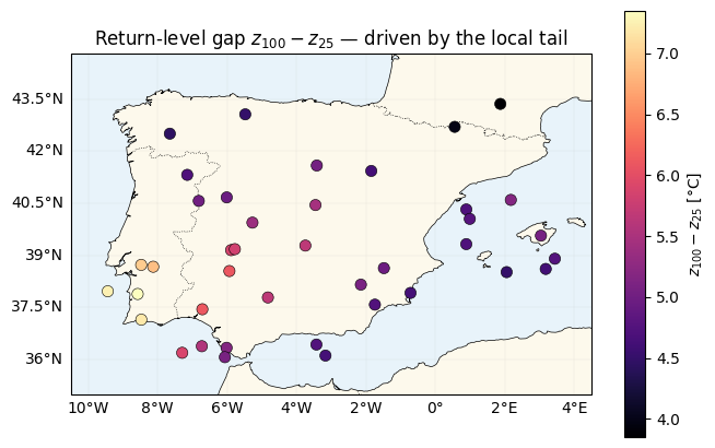

Contrast with nb 02¶

Aspect	nb 02 (multiplicative)	nb 03 (non-stationary tail)
Latent fields	$\mu(s)$ , $\tilde\beta(s)$	$\mu(s)$ , $\tilde\beta(s)$ , $\widetilde{\log\sigma}(s)$ , $\tilde\xi(s)$
GEV scale σ	global	$\sigma(s)$ spatial GP
GEV shape ξ	global	$\xi(s)$ spatial GP
$z_{100}-z_{25}$ map	~flat	spatially varying

The cost of going from two GPs to four is two more gp_sample calls and two more scalar intercepts — the inference recipe is otherwise identical.

Summary¶

Four pyrox spatial GPs feed an xtremax GEV likelihood with per-station scale and shape; NumPyro SVI infers all four fields jointly.
Centering every field + initialising the whitened GP bases at zero keeps the richer model identifiable and in-support during early SVI.
μ and σ recover well; β is modestly shrunk; ξ is the hardest (tiny signal, strong prior shrinkage) — an honest reflection of how little 40 years of maxima say about the tail shape.
The return-level gap $z_{100}-z_{25}$ now carries spatial structure from the local tail — impossible under the global-tail models of nb 01–02.

Follow-ups¶

Cross-station dependence — a Gaussian copula on the residuals (nb 04).
Temporal non-stationarity in $\sigma, \xi$ — let the tail itself drift with GMST, not just space.