Kronecker GP + GEV likelihood

Annual temperature extremes over Spain — an additive space + time GP with GEV observations¶

This notebook threads together three modelling ingredients, now built on the xtremax + pyrox + gaussx stack rather than hand-rolled helpers:

Latent space + time GPs via pyrox.gp — a spatial GP $\mu(s)$ over stations and a temporal residual GP $\tau_r(t)$ over GMST, each drawn with a whitened gp_sample inside a NumPyro model.
A Generalized Extreme Value likelihood for yearly maxima — supplied by xtremax (GeneralizedExtremeValueDistribution), so we no longer carry a bespoke numpyro.distributions.Distribution subclass.
Variational inference with a NumPyro AutoNormal guide and an optax optimiser — the mean-field posterior is learned by SVI, replacing the hand-written VariationalFactor / closed-form-KL / Gauss–Hermite-ELL loop.

The pedagogical payoff is unchanged: return-level maps — the temperature exceeded once every 25 or 100 years — at current and warming-projected climates, computed with xtremax.gev_return_level.

Background¶

Block maxima and the GEV distribution¶

Let $X_1, \dots, X_n$ be i.i.d. draws from some well-behaved base distribution and set $M_n = \max_i X_i$ . The Fisher–Tippett–Gnedenko theorem says the only non-degenerate limits of normalised $M_n$ are Generalized Extreme Value laws,

\mathrm{GEV}(y \mid \mu, \sigma, \xi) = \frac{1}{\sigma}\,\bigl[1 + \xi\,z\bigr]_+^{-(1 + 1/\xi)}\,\exp\!\Bigl(-\bigl[1 + \xi z\bigr]_+^{-1/\xi}\Bigr), \qquad z = \frac{y - \mu}{\sigma},

((1))

with $\xi > 0$ Fréchet (heavy tail), $\xi = 0$ Gumbel, $\xi < 0$ Weibull (bounded above). Mediterranean max-temperature data typically gives $\xi \in [0.05, 0.25]$ . xtremax ships this distribution and its quantile / return-level functions, matching scipy.stats.genextreme (with c = -\xi) to machine precision — we verify that below.

Additive separable structure¶

We treat space and time as two independent zero-mean GPs with no interaction, $f(s, t) = \mu_0 + \mu(s) + \tau(t)$ , and split the temporal part into a linear warming response plus a smooth residual,

\tau(t) = \beta\,\bigl(\mathrm{GMST}(t) - \overline{\mathrm{GMST}}\bigr) + \tau_r(t), \qquad \tau_r \sim \mathcal{GP}(0, k_t).

((2))

Fixing the level on $\mu_0$ and the trend on β — by centering the two GP fields to be zero-mean — removes the additive identifiability ( $\mu_0$ vs the mean of $\mu(s)$ ; β vs the mean of $\tau_r$ ) that otherwise lets the latent fields silently absorb the constant and the slope.

Setup¶

import time

import jax
import jax.numpy as jnp
import jax.random as jr
import matplotlib.pyplot as plt
import numpy as np
import optax
import cartopy.crs as ccrs
import cartopy.feature as cfeature
import numpyro
import numpyro.distributions as dist
from numpyro.infer import SVI, Predictive, Trace_ELBO, autoguide
from numpyro.infer.initialization import init_to_value
from jaxtyping import Array, Float
from scipy.stats import genextreme

# pyrox provides the GP prior + whitened latent sampling and the kernel maths;
# xtremax provides the GEV distribution and return-level helpers.
from pyrox.gp import GPPrior, Matern, RBF, gp_sample
from xtremax import GeneralizedExtremeValueDistribution as GEV
from xtremax import gev_return_level
from xtremax.simulations import generate_gmst_trajectory, generate_spatial_field

jax.config.update("jax_enable_x64", True)

/home/user/research_notebook/projects/gaussian_processes/.venv/lib/python3.12/site-packages/tqdm/auto.py:21: TqdmWarning: IProgress not found. Please update jupyter and ipywidgets. See https://ipywidgets.readthedocs.io/en/stable/user_install.html
  from .autonotebook import tqdm as notebook_tqdm

Synthetic data — a warming Spain¶

Stations¶

Forty on-land Iberian stations from xtremax.simulations.generate_spatial_field (lat/lon/elevation). In a real study you’d load AEMET or ERA5 yearly maxima — the inference below is unchanged.

SPAIN_BBOX = (-9.5, 3.5, 36.0, 43.8)  # lon_min, lon_max, lat_min, lat_max

S = 40  # number of stations
T = 40  # number of years
YEAR_0 = 1985
YEARS = jnp.arange(YEAR_0, YEAR_0 + T)

# Stations from xtremax.simulations — on-land Iberian sites (lat/lon/elevation).
_field = generate_spatial_field(n_sites=S, bounds=SPAIN_BBOX, seed=2024)
stations = jnp.stack([jnp.asarray(_field.lon.values), jnp.asarray(_field.lat.values)], axis=1)
lon_st, lat_st = stations[:, 0], stations[:, 1]

key = jr.PRNGKey(2024)

GMST proxy¶

A synthetic GMST anomaly from xtremax.simulations.generate_gmst_trajectory (linear warming trend + noise). The anomaly feeds the temporal GP.

gmst = jnp.asarray(
    generate_gmst_trajectory(
        n_years=T, start_year=YEAR_0, trend_type="linear", noise_std=0.05, seed=2024
    ).values
)
gmst_c = gmst - jnp.mean(gmst)
print(f"GMST: start {float(gmst[0]):.2f} °C  →  end {float(gmst[-1]):.2f} °C")

GMST: start 0.15 °C  →  end 0.90 °C

Ground-truth field¶

A single ground-truth realisation of the additive model, drawn from pyrox GP priors with fixed kernels via GPPrior.sample — no bespoke draw helper.

TRUTH = {
    "mu0": 35.0,
    "k_s_var": 4.0,
    "k_s_ls": 2.0,
    "k_t_var": 0.02,
    "k_t_ls": 0.25,
    "beta_gmst": 1.5,  # °C extremes per °C GMST anomaly
    "gev_sigma": 1.8,
    "gev_xi": 0.12,  # Fréchet regime
}

# Ground-truth fields drawn from pyrox GP priors (zero-mean) via GPPrior.sample.
key, key_mu, key_tau = jr.split(key, 3)
mu_truth = GPPrior(
    kernel=Matern(init_variance=TRUTH["k_s_var"], init_lengthscale=TRUTH["k_s_ls"], nu=1.5),
    X=stations,
).sample(key_mu)  # (S,) — zero-mean spatial offset
tau_resid = GPPrior(
    kernel=RBF(init_variance=TRUTH["k_t_var"], init_lengthscale=TRUTH["k_t_ls"]),
    X=gmst[:, None],
).sample(key_tau)
tau_truth = TRUTH["beta_gmst"] * gmst_c + tau_resid  # (T,)
f_truth = TRUTH["mu0"] + mu_truth[:, None] + tau_truth[None, :]  # (S, T)

GEV observation model — from `xtremax`¶

We use xtremax.GeneralizedExtremeValueDistribution directly (Coles parameterisation, $1 + \xi z$ ). Verify it matches scipy.stats.genextreme with c = -\xi across the Fréchet, Gumbel, and Weibull regimes.

y_grid = jnp.linspace(-2.0, 25.0, 60)
loc_, scale_ = 3.0, 1.5
for xi_test in [0.2, 0.0, -0.2]:
    ours = GEV(loc=loc_, scale=scale_, concentration=xi_test).log_prob(y_grid)
    theirs = genextreme.logpdf(np.asarray(y_grid), c=-xi_test, loc=loc_, scale=scale_)
    mask = np.isfinite(theirs)
    diff = float(jnp.max(jnp.abs(ours[mask] - theirs[mask])))
    print(f"xtremax GEV vs scipy  (ξ={xi_test:+.1f}):  max|Δ| = {diff:.2e}")

xtremax GEV vs scipy  (ξ=+0.2):  max|Δ| = 5.12e-13
xtremax GEV vs scipy  (ξ=+0.0):  max|Δ| = 1.42e-14

xtremax GEV vs scipy  (ξ=-0.2):  max|Δ| = 5.33e-15

Draw the observations¶

key, key_obs = jr.split(key)
y_obs = GEV(loc=f_truth, scale=TRUTH["gev_sigma"], concentration=TRUTH["gev_xi"]).sample(key_obs)
Y_MEAN = float(jnp.mean(y_obs))  # module-level constant for the mu0 prior
print(f"observations shape: {y_obs.shape}  range: [{float(y_obs.min()):.1f}, {float(y_obs.max()):.1f}] °C")

observations shape: (40, 40)  range: [27.6, 62.0] °C

Data inspection — stations + a few timeseries¶

def plot_stations(ax, values: Float[Array, " S"], *, cmap: str, vlim: tuple, label: str) -> None:
    ax.set_extent([SPAIN_BBOX[0] - 1, SPAIN_BBOX[1] + 1, SPAIN_BBOX[2] - 1, SPAIN_BBOX[3] + 1], crs=ccrs.PlateCarree())
    ax.add_feature(cfeature.COASTLINE, linewidth=0.5)
    ax.add_feature(cfeature.BORDERS, linestyle=":", linewidth=0.5)
    ax.add_feature(cfeature.OCEAN, facecolor="#e8f3fa")
    ax.add_feature(cfeature.LAND, facecolor="#fdf9ec")
    sc = ax.scatter(
        np.asarray(lon_st), np.asarray(lat_st), c=np.asarray(values), cmap=cmap,
        vmin=vlim[0], vmax=vlim[1], s=55, edgecolors="k", linewidths=0.4,
        transform=ccrs.PlateCarree(), zorder=5,
    )
    gl = ax.gridlines(draw_labels=True, linewidth=0.2, alpha=0.4)
    gl.top_labels = gl.right_labels = False
    plt.colorbar(sc, ax=ax, shrink=0.75, label=label)


fig = plt.figure(figsize=(13, 5))
ax_map = fig.add_subplot(1, 2, 1, projection=ccrs.PlateCarree())
plot_stations(ax_map, mu_truth, cmap="RdBu_r", vlim=(-5, 5), label="true μ(s) [°C]")
ax_map.set_title("Ground-truth spatial offset")

order_by_lat = jnp.argsort(lat_st)
picks = jnp.array([order_by_lat[i] for i in (0, S // 3, 2 * S // 3, S - 1)])
ax_ts = fig.add_subplot(1, 2, 2)
for s in picks:
    s_int = int(s)
    ax_ts.plot(YEARS, y_obs[s_int, :], "o-", lw=1.3, ms=4, alpha=0.8,
               label=f"({float(lat_st[s_int]):.2f}°N, {float(lon_st[s_int]):.2f}°E)")
ax_ts.set_xlabel("year")
ax_ts.set_ylabel("yearly max [°C]")
ax_ts.set_title("Observed yearly maxima — 4 stations")
ax_ts.legend(loc="upper left", fontsize=9)
ax_ts.grid(alpha=0.3)
plt.tight_layout()
plt.show()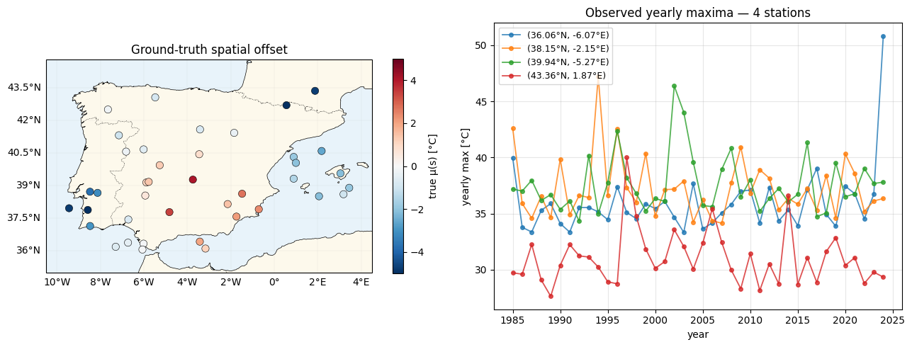

The model — pyrox GP latents + xtremax GEV likelihood¶

A single NumPyro model:

Matern-3/2 spatial kernel and RBF temporal kernel from pyrox.gp, each with log-normal hyperpriors;
latent fields drawn with whitened gp_sample (well-conditioned reparam), then centered so $\mu_0$ owns the level and β owns the trend;
an xtremax GEV likelihood on the $S \times T$ grid of yearly maxima.

def model(stations, gmst, y=None):
    gmst_c = gmst - jnp.mean(gmst)

    k_s = Matern(nu=1.5)
    k_s.set_prior("variance", dist.LogNormal(jnp.log(2.0), 0.5))
    k_s.set_prior("lengthscale", dist.LogNormal(jnp.log(2.0), 0.5))
    k_t = RBF()
    k_t.set_prior("variance", dist.LogNormal(jnp.log(0.05), 0.5))
    k_t.set_prior("lengthscale", dist.LogNormal(jnp.log(0.5), 0.5))

    mu_s = gp_sample("mu_s", GPPrior(kernel=k_s, X=stations), whitened=True)
    tau_r = gp_sample("tau_r", GPPrior(kernel=k_t, X=gmst[:, None]), whitened=True)
    # Center to remove the additive degeneracies (level → mu0, trend → beta).
    mu_s = mu_s - jnp.mean(mu_s)
    tau_r = tau_r - jnp.mean(tau_r)

    mu0 = numpyro.sample("mu0", dist.Normal(Y_MEAN, 5.0))
    beta = numpyro.sample("beta", dist.Normal(1.0, 1.0))
    log_sigma = numpyro.sample("log_sigma", dist.Normal(jnp.log(2.0), 0.4))
    xi = numpyro.sample("xi", dist.Normal(0.1, 0.1))
    sigma = jnp.exp(log_sigma)

    tau_total = beta * gmst_c + tau_r  # full temporal effect
    loc = mu0 + mu_s[:, None] + tau_total[None, :]

    numpyro.deterministic("mu_field", mu_s)        # centered spatial offset
    numpyro.deterministic("tau_total", tau_total)  # trend + residual
    numpyro.deterministic("sigma", sigma)
    numpyro.sample("y", GEV(loc=loc, scale=sigma, concentration=xi), obs=y)

Inference — SVI with a NumPyro `AutoNormal` guide¶

optax.zero_nans() guards against the occasional out-of-support GEV draw (a -inf log-prob → NaN gradient) during early exploration; init_to_value starts the location near the data so we don’t begin deep out of support.

guide = autoguide.AutoNormal(
    model,
    init_loc_fn=init_to_value(
        values={"mu0": Y_MEAN, "beta": 1.0, "log_sigma": float(jnp.log(2.0)), "xi": 0.1}
    ),
)
optimizer = numpyro.optim.optax_to_numpyro(
    optax.chain(optax.zero_nans(), optax.clip_by_global_norm(10.0), optax.adam(3e-3))
)
svi = SVI(model, guide, optimizer, Trace_ELBO())

t0 = time.time()
svi_result = svi.run(jr.PRNGKey(0), 5000, stations, gmst, y_obs, progress_bar=False)
losses = np.asarray(svi_result.losses)
print(f"SVI finished in {time.time() - t0:.1f}s")

# Posterior draws: deterministics via Predictive, scalar latents via the guide.
post = Predictive(model, guide=guide, params=svi_result.params, num_samples=600)(
    jr.PRNGKey(3), stations, gmst
)
lat = guide.sample_posterior(jr.PRNGKey(4), svi_result.params, sample_shape=(600,))

print(f"fitted μ₀  = {float(lat['mu0'].mean()):.2f} ± {float(lat['mu0'].std()):.2f}  (truth {TRUTH['mu0']})")
print(f"fitted β   = {float(lat['beta'].mean()):.2f} ± {float(lat['beta'].std()):.2f}  (truth {TRUTH['beta_gmst']})")
print(f"fitted σ   = {float(post['sigma'].mean()):.2f} ± {float(post['sigma'].std()):.2f}  (truth {TRUTH['gev_sigma']})")
print(f"fitted ξ   = {float(lat['xi'].mean()):.3f} ± {float(lat['xi'].std()):.3f}  (truth {TRUTH['gev_xi']})")

SVI finished in 13.3s

fitted μ₀  = 34.41 ± 0.05  (truth 35.0)
fitted β   = 1.18 ± 0.17  (truth 1.5)
fitted σ   = 1.83 ± 0.04  (truth 1.8)
fitted ξ   = 0.142 ± 0.021  (truth 0.12)

Loss curve¶

fig, ax = plt.subplots(figsize=(10, 3.2))
finite = np.isfinite(losses)
ax.plot(np.arange(len(losses))[finite], losses[finite], "C3-", lw=1.2)
ax.set_xlabel("SVI step")
ax.set_ylabel("−ELBO")
ax.set_yscale("symlog", linthresh=100.0)
ax.set_title("SVI training — pyrox GP latents + xtremax GEV likelihood")
ax.grid(alpha=0.3, which="both")
plt.show()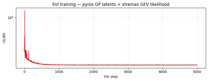

Parameter recovery¶

The additive model has a residual constant degeneracy between $\mu_0$ and the mean of $\mu(s)$ ; with the centered fields the posterior tracks the truth’s shape with a small (≲ 0.5 °C) vertical offset.

m_s_fit = post["mu_field"].mean(0)
v_s_fit = post["mu_field"].std(0)
tau_fit = post["tau_total"].mean(0)
tau_sd = post["tau_total"].std(0)
tau_truth_c = tau_truth - jnp.mean(tau_truth)  # compare zero-mean temporal effects

fig, axes = plt.subplots(1, 2, figsize=(13, 4.2))
ax = axes[0]
order_s = jnp.argsort(mu_truth)
x = jnp.arange(S)
ax.plot(x, mu_truth[order_s], "ko", ms=6, label="truth", zorder=3)
ax.errorbar(x, m_s_fit[np.asarray(order_s)], yerr=2 * v_s_fit[np.asarray(order_s)],
            fmt="rD", ms=4, alpha=0.7, label=r"posterior $\pm 2\sigma$", capsize=2)
ax.set_xlabel("station (sorted by truth)")
ax.set_ylabel("μ(s) [°C]")
ax.set_title("Recovered spatial offsets (centered)")
ax.legend()
ax.grid(alpha=0.3)

ax = axes[1]
ax.plot(YEARS, tau_truth_c, "k-", lw=2, label="truth", zorder=3)
ax.plot(YEARS, tau_fit, "r-", lw=2, label="posterior mean")
ax.fill_between(YEARS, tau_fit - 2 * tau_sd, tau_fit + 2 * tau_sd, alpha=0.25, color="red", label=r"$\pm 2\sigma$")
ax.set_xlabel("year")
ax.set_ylabel("τ(t) − mean [°C]")
ax.set_title("Recovered temporal effect (trend + residual)")
ax.legend()
ax.grid(alpha=0.3)
plt.tight_layout()
plt.show()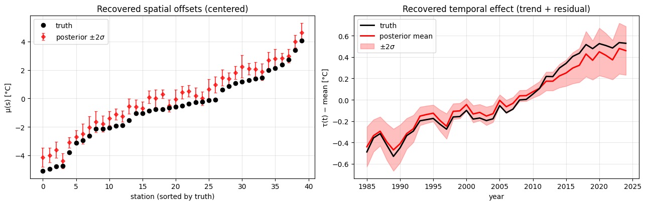

GEV tail recovery¶

fig, axes = plt.subplots(1, 2, figsize=(11, 3.8))
for ax, (name, truth_val, draws, xr) in zip(
    axes,
    [("σ (GEV scale)", TRUTH["gev_sigma"], post["sigma"], (1.0, 2.6)),
     ("ξ (GEV shape)", TRUTH["gev_xi"], lat["xi"], (-0.05, 0.3))],
    strict=True,
):
    ax.hist(np.asarray(draws).ravel(), bins=40, color="C0", alpha=0.6, density=True)
    ax.axvline(truth_val, color="k", ls="--", lw=2, label="truth")
    ax.axvline(float(np.mean(draws)), color="red", lw=2, label="posterior mean")
    ax.set_xlim(*xr)
    ax.set_title(name)
    ax.legend(loc="upper right")
    ax.grid(alpha=0.3)
plt.tight_layout()
plt.show()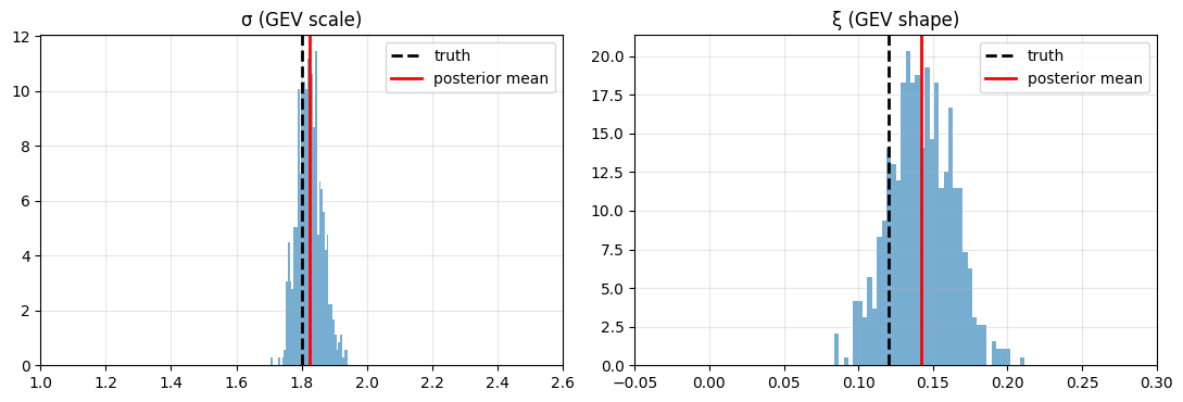

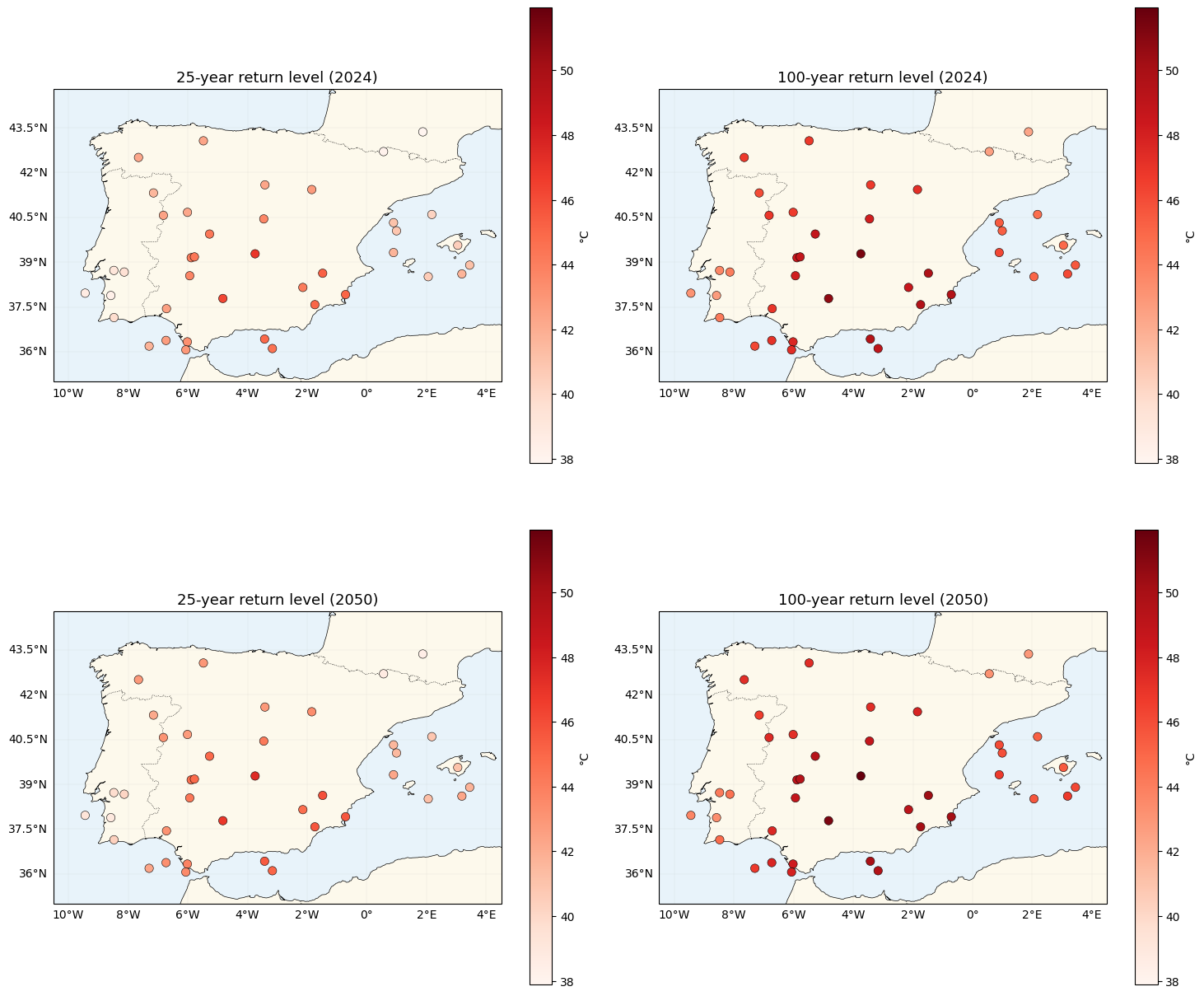
The payoff — return-level maps¶

The $T_r$ -year return level is $z_p = F^{-1}(1 - 1/T_r)$ , computed with xtremax.gev_return_level. We map 25- and 100-year return temperatures for a typical year at the end of record (2024) and a warming projection (2050) obtained by linearly extrapolating GMST.

mu_field_mean = post["mu_field"].mean(0)  # (S,)
mu0_p = float(lat["mu0"].mean())
beta_p = float(lat["beta"].mean())
sigma_p = float(post["sigma"].mean())
xi_p = float(lat["xi"].mean())

gmst_2024 = gmst[-1]
gmst_2050 = gmst[-1] + (gmst[-1] - gmst[0]) / (T - 1) * (2050 - (YEAR_0 + T - 1))
print(f"GMST 2024 = {float(gmst_2024):.3f} °C, GMST 2050 (extrapolated) = {float(gmst_2050):.3f} °C")

loc_2024 = mu0_p + mu_field_mean + beta_p * (gmst_2024 - jnp.mean(gmst))
loc_2050 = mu0_p + mu_field_mean + beta_p * (gmst_2050 - jnp.mean(gmst))

z25_2024 = gev_return_level(25.0, loc_2024, sigma_p, xi_p)
z100_2024 = gev_return_level(100.0, loc_2024, sigma_p, xi_p)
z25_2050 = gev_return_level(25.0, loc_2050, sigma_p, xi_p)
z100_2050 = gev_return_level(100.0, loc_2050, sigma_p, xi_p)

stacked = jnp.stack([z25_2024, z100_2024, z25_2050, z100_2050])
vmin, vmax = float(jnp.min(stacked)), float(jnp.max(stacked))
print(f"2024 → 2050 mean shift in 100-yr return level: "
      f"{float(jnp.mean(z100_2050) - jnp.mean(z100_2024)):.2f} °C")

fig, axes = plt.subplots(2, 2, figsize=(15, 14), subplot_kw={"projection": ccrs.PlateCarree()})
for ax, values, title in zip(
    axes.flat,
    [z25_2024, z100_2024, z25_2050, z100_2050],
    ["25-year return level (2024)", "100-year return level (2024)",
     "25-year return level (2050)", "100-year return level (2050)"],
    strict=True,
):
    plot_stations(ax, values, cmap="Reds", vlim=(vmin, vmax), label="°C")
    ax.set_title(title, fontsize=13)
plt.tight_layout()
plt.show()

GMST 2024 = 0.903 °C, GMST 2050 (extrapolated) = 1.403 °C

2024 → 2050 mean shift in 100-yr return level: 0.59 °C

Summary¶

pyrox.gp supplies the kernels (Matern, RBF, matern_kernel, rbf_kernel), the GPPrior, and whitened gp_sample latent fields.
xtremax supplies the GEV likelihood (GeneralizedExtremeValueDistribution, machine-precision vs scipy) and the return-level helper (gev_return_level).
NumPyro SVI with an AutoNormal guide replaces the hand-rolled variational scaffold; centering the latent fields fixes the additive identifiability so $\mu_0$ owns the level and β owns the warming trend.

Follow-ups¶

Multiplicative $K_s \otimes K_t$ — spatially-varying warming rates.
Non-stationary GEV — let $\log\sigma$ and/or ξ vary over space.
Real data — swap the synthetic stations / maxima for AEMET or ERA5.