Spatiotemporal Preprocessing — Geo, Time, and the Pandas Pipeline

Real spatiotemporal data arrives in awkward shapes:

Geographic coordinates wrap around at $\pm 180°$ longitude and live on a sphere — a raw $(lon, lat)$ MLP has to learn the seam from scratch and never quite manages.
Time covariates carry strong periodicities (daily, weekly, yearly) that a raw scalar t cannot express compactly.
DataFrames mix all of this with column names and need a fit-once, transform-often lifecycle.

pyrox.nn and pyrox.preprocessing provide composable layers for the first two concerns and a pandas-side facade for the third. This notebook walks through:

Geographic encoders — Deg2Rad, Cartesian3DEncoder, SphericalHarmonicEncoder, LonLatScale. Same downstream MLP, different encoders — show the seam vanish.
Time / seasonal encoders — FourierFeatures, SeasonalFeatures and the underlying pure-JAX helpers. A linear regression on encoded time fits multiperiodic signals.
Pandas-side fit_spatiotemporal — one call builds a fitted bundle of layers from a DataFrame; the bundle re-encodes test rows with the same time_min.

Setup¶

import subprocess
import sys


try:
    import google.colab  # noqa: F401

    IN_COLAB = True
except ImportError:
    IN_COLAB = False

if IN_COLAB:
    subprocess.run(
        [
            sys.executable,
            "-m",
            "pip",
            "install",
            "-q",
            "pyrox[colab] @ git+https://github.com/jejjohnson/pyrox@main",
        ],
        check=True,
    )

import warnings


warnings.filterwarnings("ignore", message=r".*IProgress.*")

import equinox as eqx
import jax
import jax.numpy as jnp
import jax.random as jr
import matplotlib.pyplot as plt
import numpy as np
import optax
import pandas as pd

from pyrox.nn import (
    Cartesian3DEncoder,
    Deg2Rad,
    LonLatScale,
    SeasonalFeatures,
    SphericalHarmonicEncoder,
    seasonal_features,
    spherical_harmonic_encode,
)
from pyrox.preprocessing import encode_time_column, fit_spatiotemporal


jax.config.update("jax_enable_x64", True)

import importlib.util


try:
    from IPython import get_ipython

    ipython = get_ipython()
except ImportError:
    ipython = None

if ipython is not None and importlib.util.find_spec("watermark") is not None:
    ipython.run_line_magic("load_ext", "watermark")
    ipython.run_line_magic(
        "watermark",
        "-v -m -p jax,equinox,numpyro,pyrox,pandas,matplotlib",
    )
else:
    print("watermark extension not installed; skipping reproducibility readout.")

Python implementation: CPython
Python version       : 3.13.5
IPython version      : 9.10.0

jax       : 0.9.2
equinox   : 0.13.6
numpyro   : 0.20.1
pyrox     : 0.0.6
pandas    : 3.0.2
matplotlib: 3.10.8

Compiler    : GCC 11.2.0
OS          : Linux
Release     : 6.8.0-1044-azure
Machine     : x86_64
Processor   : x86_64
CPU cores   : 16
Architecture: 64bit

1. Geographic encoders — the lon/lat seam¶

The seam, formally¶

Geographic coordinates parameterise the sphere as

\Phi : [-180°, 180°] \times [-90°, 90°] \to S^2, \qquad (\lambda, \phi) \mapsto (\cos\phi\cos\lambda,\ \cos\phi\sin\lambda,\ \sin\phi).

((1))

This map is not injective at the boundary:

$\Phi(-180°, \phi) = \Phi(+180°, \phi)$ for every ϕ (the antimeridian — the date line),
$\Phi(\lambda, +90°)$ is the same point for every λ (the north pole; analogously the south pole).

A raw $(\lambda, \phi)$ MLP sees the chart, not the sphere: $\lambda = -180°$ and $\lambda = +180°$ are the two ends of a $360°$ -wide interval, and the model has no built-in notion that they are the same physical point. Two costs follow:

Discontinuity at the antimeridian. A continuous function $f : S^2 \to \mathbb{R}$ pulled back to the chart need not be continuous in λ at $\pm 180°$ — a function value $f(\lambda^\star)$ near the date line has nothing constraining it from the “other side.” A standard MLP has to learn the equivalence from data.
Polar singularity. At $\phi = \pm 90°$ , the entire interval $\lambda \in [-180°, 180°]$ collapses to a single point, so the angular metric is wildly distorted near the poles.

The fix is to compose with Φ and feed the unit-Cartesian coordinates instead:

x \in S^2 \subset \mathbb{R}^3, \qquad x = (\cos\phi \cos\lambda,\ \cos\phi \sin\lambda,\ \sin\phi),\ \ \|x\|_2 = 1.

((2))

pyrox.nn.Cartesian3DEncoder is exactly Φ. Both date-line points land on the same $x$ , and the polar singularity disappears (the north and south poles are simply $(0, 0, \pm 1)$ ).

From $S^2$ to a smooth basis: real spherical harmonics¶

$\mathbb{R}^3$ -coordinates are continuous on the sphere, but for regression we usually want an orthonormal basis of $L^2(S^2)$ — the spherical analogue of the Fourier basis on a circle. The real spherical harmonics $\{Y_\ell^m\}$ for degree $\ell \ge 0$ and order $m \in \{-\ell, \ldots, \ell\}$ are

Y_\ell^m(\theta, \phi) = \begin{cases} \sqrt{2}\, N_\ell^{|m|}\, P_\ell^{|m|}(\cos\theta)\,\sin(|m|\,\phi) & m < 0, \\ N_\ell^0\, P_\ell^0(\cos\theta) & m = 0, \\ \sqrt{2}\, N_\ell^m\, P_\ell^m(\cos\theta)\,\cos(m\,\phi) & m > 0, \end{cases} \qquad N_\ell^m = \sqrt{\frac{(2\ell + 1)(\ell - m)!}{4\pi (\ell + m)!}},

((3))

where $P_\ell^m$ is the associated Legendre polynomial and $(\theta, \phi) = (\pi/2 - \phi_{\mathrm{lat}},\, \lambda)$ are the colatitude / longitude angles. Truncating at $\ell \le \ell_\text{max}$ gives a basis of dimension $(\ell_\text{max} + 1)^2$ — a spherical analogue of a band-limited Fourier basis. SphericalHarmonicEncoder(l_max=3) produces $(\ell_\text{max} + 1)^2 = 16$ features.

Any square-integrable function on the sphere expands as $f(x) = \sum_{\ell, m} c_{\ell, m}\, Y_\ell^m(x)$ , so a linear head on truncated SH features is the optimal least-squares fit when the target lies in that span — which is exactly the experiment we run below.

We build a synthetic target that’s a low-degree real spherical harmonic so we know the right basis to fit it.

key_loc = jr.PRNGKey(0)
n_train = 2000
lon_deg = jr.uniform(key_loc, (n_train,), minval=-180.0, maxval=180.0)
lat_deg = jr.uniform(jr.fold_in(key_loc, 1), (n_train,), minval=-89.0, maxval=89.0)
lonlat_deg_train = jnp.stack([lon_deg, lat_deg], axis=-1)

# Ground-truth signal: a fixed linear combination of degree-2 / degree-3 SHs.
sh_train = spherical_harmonic_encode(
    Deg2Rad()(lonlat_deg_train), l_max=3, input_unit="radians"
)  # (N, 16)
true_coeffs = jr.normal(jr.PRNGKey(42), (16,))
y_train = sh_train @ true_coeffs

def make_pipeline_raw() -> eqx.nn.MLP:
    """Pipeline 1 — feed (lon, lat) in degrees, scaled to [-1, 1], straight to an MLP."""
    return eqx.nn.MLP(
        in_size=2,
        out_size=1,
        width_size=64,
        depth=3,
        activation=jax.nn.tanh,
        key=jr.PRNGKey(7),
    )


class SpherePipeline(eqx.Module):
    """Pipeline 2 — Deg2Rad → Cartesian3D → SH features → linear head."""

    sh_encoder: SphericalHarmonicEncoder
    head: eqx.nn.Linear

    def __call__(self, lonlat_deg: jax.Array) -> jax.Array:
        radians = Deg2Rad()(lonlat_deg)
        cart = Cartesian3DEncoder(input_unit="radians")(radians)
        feats = self.sh_encoder(cart)
        return jax.vmap(self.head)(feats)[..., 0]


def make_pipeline_sphere() -> SpherePipeline:
    sh = SphericalHarmonicEncoder(l_max=3, input_mode="cartesian")
    return SpherePipeline(
        sh_encoder=sh,
        head=eqx.nn.Linear(sh.num_features, 1, key=jr.PRNGKey(8)),
    )

Both pipelines have comparable parameter counts (the MLP has more if anything), so any difference in test loss is the encoder, not the capacity.

def fit(model, x: jax.Array, y: jax.Array, *, lr: float, n_steps: int):
    optim = optax.adam(lr)
    state = optim.init(eqx.filter(model, eqx.is_inexact_array))

    @eqx.filter_jit
    def step(m, s):
        def loss_fn(p):
            preds = jax.vmap(p)(x) if isinstance(p, eqx.nn.MLP) else p(x)
            preds = preds.reshape(-1) if preds.ndim > 1 else preds
            return jnp.mean((preds - y) ** 2)

        loss, grads = eqx.filter_value_and_grad(loss_fn)(m)
        updates, ns = optim.update(grads, s, eqx.filter(m, eqx.is_inexact_array))
        return eqx.apply_updates(m, updates), ns, loss

    losses = []
    for _ in range(n_steps):
        model, state, loss = step(model, state)
        losses.append(float(loss))
    return model, jnp.asarray(losses)


# Scale lon/lat into [-1, 1] before feeding the raw MLP — gives it a fair shot.
scaler = LonLatScale()
mlp_raw = make_pipeline_raw()
mlp_raw, raw_losses = fit(
    mlp_raw, scaler(lonlat_deg_train), y_train, lr=3e-3, n_steps=2000
)

mlp_sphere = make_pipeline_sphere()
mlp_sphere, sphere_losses = fit(
    mlp_sphere, lonlat_deg_train, y_train, lr=3e-3, n_steps=2000
)

print(f"Raw (lon,lat) MLP final MSE:  {float(raw_losses[-1]):.4f}")
print(f"Sphere SH-encoder MSE:        {float(sphere_losses[-1]):.4e}")

Raw (lon,lat) MLP final MSE:  0.0003
Sphere SH-encoder MSE:        3.8223e-06

The spherical-harmonic head fits to numerical zero in 2000 steps — it has the right basis. The raw $(lon, lat)$ MLP plateaus several orders of magnitude higher because it has to discover the wraparound and the spherical basis from scratch.

Let’s look at where the residual error lives on the globe.

n_grid = 64
lon_grid = jnp.linspace(-180.0, 180.0, 2 * n_grid)
lat_grid = jnp.linspace(-89.0, 89.0, n_grid)
LON, LAT = jnp.meshgrid(lon_grid, lat_grid, indexing="xy")
grid_lonlat = jnp.stack([LON.ravel(), LAT.ravel()], axis=-1)

sh_grid = spherical_harmonic_encode(
    Deg2Rad()(grid_lonlat), l_max=3, input_unit="radians"
)
y_grid = (sh_grid @ true_coeffs).reshape(LON.shape)
y_raw = jax.vmap(mlp_raw)(scaler(grid_lonlat))[:, 0].reshape(LON.shape)
y_sphere = mlp_sphere(grid_lonlat).reshape(LON.shape)

fig, axes = plt.subplots(1, 3, figsize=(18, 5))
extent = (-180, 180, -89, 89)
im0 = axes[0].imshow(np.asarray(y_grid), extent=extent, origin="lower", cmap="RdBu_r")
axes[0].set_title("Truth — degree-3 SH combination")
plt.colorbar(im0, ax=axes[0], fraction=0.025)
im1 = axes[1].imshow(
    np.asarray(jnp.abs(y_raw - y_grid)), extent=extent, origin="lower", cmap="magma"
)
axes[1].set_title("|truth − raw (lon,lat) MLP|")
plt.colorbar(im1, ax=axes[1], fraction=0.025)
im2 = axes[2].imshow(
    np.asarray(jnp.abs(y_sphere - y_grid)),
    extent=extent,
    origin="lower",
    cmap="magma",
)
axes[2].set_title("|truth − sphere SH encoder|")
plt.colorbar(im2, ax=axes[2], fraction=0.025)
for ax in axes:
    ax.set_xlabel("longitude (°)")
    ax.set_ylabel("latitude (°)")
plt.show()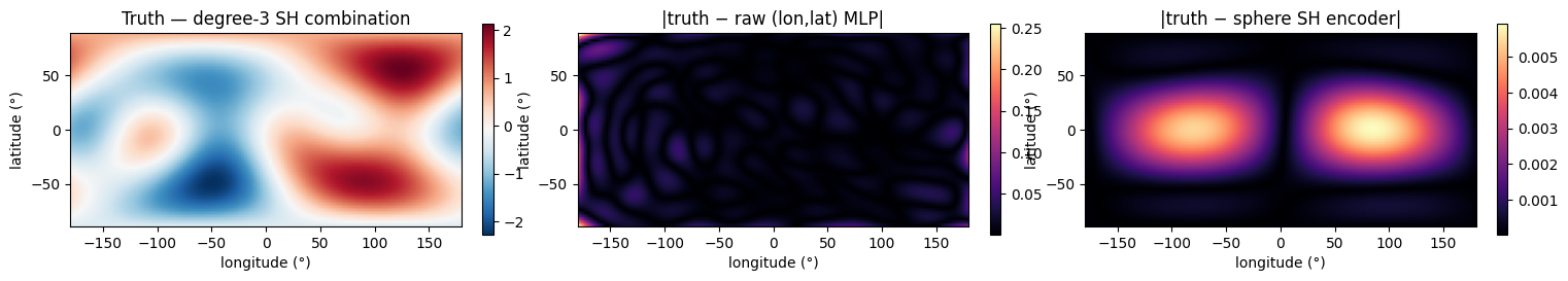

The raw MLP’s residual concentrates near $\lambda = \pm 180°$ (the seam) and at the poles — exactly the regions where a flat $(lon, lat)$ representation lies most about the underlying geometry. The spherical-harmonic encoder makes the seam invisible.

2. Time encoders — periodic signals¶

Seasonal features = truncated Fourier series on a circle¶

A function with known period τ is a function on the circle $\mathbb{R} / \tau\mathbb{Z}$ , and its Fourier series is

f(t) = a_0 + \sum_{h=1}^\infty \Bigl[a_h \cos(2\pi h t / \tau) + b_h \sin(2\pi h t / \tau)\Bigr].

((4))

Truncating at $h = H$ gives a $2H + 1$ -dimensional basis that exactly represents the band-limited part of $f$ . When several periods $\tau_1, \ldots, \tau_P$ are present (daily, weekly, yearly) the joint basis is a direct sum:

\Phi(t) = \bigoplus_{p=1}^P \bigl\{\cos(2\pi h t / \tau_p),\ \sin(2\pi h t / \tau_p)\bigr\}_{h=1}^{H_p},

((5))

of dimension $\sum_p 2 H_p$ . pyrox.nn.SeasonalFeatures(periods=(τ_1, …, τ_P), harmonics=(H_1, …, H_P)) is exactly this Φ. No constant column — add a separate intercept if you want one.

Once $f \approx \Phi(t)\, \beta$ is linear in $\beta \in \mathbb{R}^{2 \sum H_p}$ , OLS recovers β in closed form: $\hat\beta = (\Phi^\top \Phi)^{-1} \Phi^\top y$ . No deep learning required for the periodic part of the signal.

Dyadic Fourier features for unknown frequencies¶

When the period is not known, pyrox.nn.FourierFeatures evaluates dyadic frequencies

\phi_d^{\cos}(t) = \cos(2\pi \cdot 2^d \cdot t), \qquad \phi_d^{\sin}(t) = \sin(2\pi \cdot 2^d \cdot t), \quad d = 0, 1, \ldots, D - 1,

((6))

i.e. frequencies $\{1, 2, 4, 8, \ldots, 2^{D-1}\}$ — geometrically spaced rather than linearly spaced. This is the deterministic cousin of random Fourier features (Rahimi & Recht 2007): the geometric spacing covers many decades of frequency with $D$ features instead of needing $\mathcal{O}(2^D)$ linear-spaced ones. Using rescale=True divides each pair $(\cos_d, \sin_d)$ by $d + 1$ , giving a $1/k$ -prior on frequency that biases the model toward smoother solutions.

Demo¶

We synthesize a series with two known periods (daily $\tau_1 = 24$ and weekly $\tau_2 = 168$ , in hours) and a small linear trend,

y(t) = 1.5\sin(2\pi t / 24) + 0.5\cos(4\pi t / 24) + 0.8\sin(2\pi t / 168) + 0.005\, t + \varepsilon,\qquad \varepsilon \sim \mathcal{N}(0, 0.01),

((7))

and fit it with ordinary least squares on a $\Phi(t)$ design matrix that has $H_1 = 2$ harmonics for the daily cycle, $H_2 = 1$ for the weekly cycle, plus an intercept and a trend column. Six seasonal features + 2 trend columns = an 8-dim linear model.

period_daily = 24.0
period_weekly = 168.0
n_t = 1000
t = jnp.linspace(0.0, 600.0, n_t)
y_periodic = (
    1.5 * jnp.sin(2 * jnp.pi * t / period_daily)
    + 0.5 * jnp.cos(2 * jnp.pi * 2 * t / period_daily)
    + 0.8 * jnp.sin(2 * jnp.pi * t / period_weekly)
    + 0.005 * t
)
key_eps = jr.PRNGKey(11)
y_periodic = y_periodic + 0.1 * jr.normal(key_eps, t.shape)

# Build a SeasonalFeatures layer with the right two periods.
seasonal = SeasonalFeatures(periods=(period_daily, period_weekly), harmonics=(2, 1))
phi = seasonal(t)  # (N, 2 * (2 + 1)) = (N, 6)
print(f"Seasonal feature matrix shape: {phi.shape}")

# Concatenate a trend column for the linear baseline + intercept.
X_design = jnp.concatenate([phi, t[:, None], jnp.ones_like(t)[:, None]], axis=-1)
coeffs, *_ = jnp.linalg.lstsq(X_design, y_periodic)
y_fit = X_design @ coeffs

residual = y_periodic - y_fit
print(f"In-sample R²: {1.0 - float(jnp.var(residual) / jnp.var(y_periodic)):.4f}")

Seasonal feature matrix shape: (1000, 6)

In-sample R²: 0.9955

fig, axes = plt.subplots(1, 2, figsize=(18, 5))
axes[0].plot(t[:200], y_periodic[:200], color="C1", alpha=0.6, label="observed")
axes[0].plot(t[:200], y_fit[:200], color="C0", label="seasonal-feature fit")
axes[0].set_xlabel("t")
axes[0].set_ylabel("y")
axes[0].set_title("First 200 time steps — fit vs observation")
axes[0].legend(loc="upper right")

axes[1].imshow(
    np.asarray(phi.T),
    aspect="auto",
    interpolation="nearest",
    cmap="RdBu_r",
    extent=(0, n_t, phi.shape[1], 0),
)
axes[1].set_xlabel("t (sample index)")
axes[1].set_ylabel("seasonal feature column")
axes[1].set_title("SeasonalFeatures(periods=(24, 168), harmonics=(2, 1)) — 6 columns")
plt.show()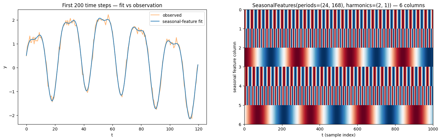

Six features explain the signal almost completely (high $R^2$ ). The feature heatmap shows the cos/sin pairs at the two daily harmonics and the single weekly cycle.

Pure-JAX helpers¶

The same encoders are exposed as pure functions in pyrox.nn (no module state, no NumPyro registration) for callers that need to compose them inside a lax.scan or a custom guide. They are what the layers above wrap internally.

phi_pure = seasonal_features(t, periods=(period_daily, period_weekly), harmonics=(2, 1))
np.testing.assert_allclose(np.asarray(phi), np.asarray(phi_pure), atol=1e-12)
print("Layer output and pure-function output match — they're literally the same math.")

Layer output and pure-function output match — they're literally the same math.

3. Pandas-side `fit_spatiotemporal`¶

Real workflows live in DataFrames. pyrox.preprocessing.fit_spatiotemporal builds a single immutable SpatiotemporalFit bundle from a DataFrame in one call. The bundle holds:

the standardization layer:
$\tilde x_{n, j} = \frac{x_{n, j} - \mu_j}{\sigma_j}, \qquad \mu_j = \tfrac{1}{N}\sum_n x_{n, j},\quad \sigma_j^2 = \tfrac{1}{N}\sum_n (x_{n, j} - \mu_j)^2,$
((8))
the requested FourierFeatures, SeasonalFeatures, and InteractionFeatures layers,
the time-axis constants $(t_{\min}, s)$ used by encode_time_column:
$\tilde t_n = s \cdot (t_n - t_{\min}),$
((9))
where $s = 1$ for integer time and $s = 1/(\text{ns per unit})$ for datetime time so that $\tilde t$ is in the unit you specified (freq="H" ⇒ hours, etc.).

The crucial invariant: at test time, re-use the same $\mu, \sigma, t_{\min}, s$ that the training-time fit produced. Re-fitting them on the test split would silently shift the encoding and corrupt the predictions. SpatiotemporalFit is equinox-immutable so the constants cannot be accidentally re-fit.

rng = np.random.default_rng(0)
n_obs = 480
times = pd.date_range("2024-01-01", periods=n_obs, freq="h")
df = pd.DataFrame(
    {
        "t": times,
        "lon": rng.uniform(-10.0, 10.0, n_obs),
        "lat": rng.uniform(40.0, 50.0, n_obs),
        "y": rng.normal(0.0, 1.0, n_obs),
    }
)
df.head()

Loading...

fit = fit_spatiotemporal(
    df,
    feature_cols=["t", "lon", "lat"],
    target_col="y",
    timetype="datetime",
    freq="H",
    seasonality_periods=(24.0, 24.0 * 7.0),  # daily, weekly (in hours)
    num_seasonal_harmonics=(3, 2),
    fourier_degrees=(0, 4, 4),  # no Fourier on time, 4 dyadic on lon/lat
    interactions=((1, 2),),  # lon × lat product
    standardize=("lon", "lat"),  # never standardize the time axis
)
print(f"time_min = {fit.time_min}")
print(f"time_scale = {fit.time_scale}")
print(f"feature_cols = {fit.feature_cols}")

time_min = 473352.0
time_scale = 2.777777777777778e-13
feature_cols = ('t', 'lon', 'lat')

Encode a held-out hour using the stored time_min so train and test align.

held_out = df.iloc[-5:]
t_train_encoded, _, _ = encode_time_column(df["t"], timetype="datetime", freq="H")
t_test_encoded, _, _ = encode_time_column(
    held_out["t"], timetype="datetime", freq="H", time_min=fit.time_min
)
print("First train rows (hours since fit.time_min):", np.asarray(t_train_encoded[:3]))
print("Held-out test rows (hours since fit.time_min):", np.asarray(t_test_encoded))

# Compose the full feature matrix for the held-out rows.
x_test = jnp.asarray(held_out[["lon", "lat"]].to_numpy(), dtype=jnp.float32)
x_test_full = jnp.concatenate([t_test_encoded[:, None], x_test], axis=-1)

standardized = fit.standardize_layer(x_test_full)
fourier = fit.fourier_layer(standardized)
seasonal_block = fit.seasonal_layer(t_test_encoded)
interactions = fit.interaction_layer(standardized)

print(
    f"Block widths — standardize:{standardized.shape[1]} "
    f"fourier:{fourier.shape[1]} "
    f"seasonal:{seasonal_block.shape[1]} "
    f"interactions:{interactions.shape[1]}"
)

First train rows (hours since fit.time_min): [0. 1. 2.]
Held-out test rows (hours since fit.time_min): [475. 476. 477. 478. 479.]

Block widths — standardize:3 fourier:16 seasonal:10 interactions:1

That SpatiotemporalFit is the building block that the BNFEstimator family (pyrox.api.BNFEstimator) consumes — but the bundle is useful on its own when you want to drive a custom model with the same standardize / Fourier / seasonal / interaction stack.

Takeaways¶

Geographic encoders absorb the chart non-injectivity of $(\lambda, \phi)$ : the date-line equivalence and the polar singularity disappear once you compose with $\Phi : (\lambda, \phi) \mapsto (\cos\phi\cos\lambda, \cos\phi\sin\lambda, \sin\phi)$ . Real spherical harmonics $\{Y_\ell^m\}_{\ell \le \ell_\text{max}}$ on top give a dimension- $(\ell_\text{max} + 1)^2$ orthonormal basis of $L^2(S^2)$ , so a linear head suffices for any band-limited spherical signal.
Seasonal / Fourier features reduce regression on a periodic time axis to OLS on a truncated Fourier basis. Use SeasonalFeatures(periods=…, harmonics=…) when the periodicities are known (the basis is exactly the truncated Fourier series on $\mathbb{R}/\tau\mathbb{Z}$ ); use FourierFeatures(degrees=D) for dyadic frequencies $\{1, 2, \ldots, 2^{D-1}\}$ when they are not.
fit_spatiotemporal keeps pandas at the boundary and freezes $(\mu_j, \sigma_j, t_{\min}, s)$ at training time as a single immutable SpatiotemporalFit of pure JAX layers + scalars. Re-use the same bundle at predict time — re-fitting any of those constants on the test split silently shifts the encoding and corrupts predictions.