Ensemble runners

Background — the runner contract and the math behind it¶

Why a class?¶

The free-function primitives (ensemble_init, ensemble_step) are intentionally minimal: they take everything as keyword arguments, return tuples, and assume nothing about your training loop. That’s great for one-off experiments and bridge code, but in production you usually want a single immutable object that bundles the configuration (log_joint, init_fn, optimizer, ensemble_size, prior_weight) so you don’t have to thread those arguments through every call site.

EnsembleMAP is that bundle. It is an equinox.Module, so it is itself a PyTree — JIT-friendly, picklable, and safe to pass across function boundaries — and it exposes exactly three methods, each mirroring numpyro.infer.SVI:

MAP as a fixed-point of the score¶

Per ensemble member, MAP solves

equivalently a fixed-point of the regularized score function:

SGD with a small enough learning rate is a discrete-time approximation of gradient flow on this potential, and Adam is the same flow with per-coordinate adaptive preconditioning by exponentially-weighted estimates of the gradient’s first and second moments.

VI as KL minimization¶

VI replaces the intractable posterior $p(\theta \mid y, x) \propto p(y \mid x, \theta)\,p(\theta)$ with a tractable surrogate $q_{\phi}(\theta)$ from a parametric family (here: mean-field Gaussian, via NumPyro’s AutoNormal). The variational parameters ϕ are chosen to minimize the reverse KL divergence,

where the evidence lower bound is

The first term is the expected log-likelihood under $q_\phi$; the second is the KL between the surrogate and the prior, acting as regularization toward the prior. The two terms are estimated by Monte-Carlo over $S$ samples $\theta^{(s)} \sim q_\phi$ (the num_particles argument). EnsembleVI exposes a kl_weight β that scales the KL term — $\beta = 1$ recovers the standard ELBO, $\beta < 1$ gives a cold posterior tempering that often improves predictive calibration on neural-scale models (Wenzel et al., 2020).

MAP versus VI in one line — Dirac vs Gaussian per member¶

EnsembleMAP and EnsembleVI differ only in what each member fits. MAP fits a point estimate per member and treats the ensemble as a uniform mixture of $E$ Dirac masses,

VI fits a mean-field Gaussian surrogate $q_{\phi_e}(\theta) = \prod_k \mathcal{N}(\theta_k \mid \mu_{e,k}, \sigma_{e,k}^2)$ per member and treats the ensemble as a mixture of $E$ Gaussians,

Posterior-predictive Monte Carlo and variance decomposition¶

Predictions for a fresh input $x^*$ come from the posterior predictive

For the ensemble surrogates above, this collapses to a Monte-Carlo estimator over the relevant axes:

The MAP estimator iterates over $E$ point masses; the VI estimator iterates over $E \times S$ samples drawn from the variational surrogates. By the law of total variance,

For a Gaussian likelihood $\mathcal{N}(f_\theta(x^*), \sigma^2)$, the aleatoric term is just $\sigma^2$ — constant in $x^*$. For a MAP ensemble, the epistemic variance is the between-member spread $\frac{1}{E}\sum_e (f_{\hat\theta_e}(x^*) - \bar f(x^*))^2$. For a VI ensemble, the epistemic variance has two contributions: between-member spread and within-member spread (because each $q_{\phi_e}$ has nonzero variance), so the predictive bands are wider — especially in extrapolation regions where $f_\theta$’s output depends sensitively on weights that the data didn’t constrain.

Setup¶

Problem setup — the sinc dataset¶

Same data and the same noisy-test-set protocol as the primitives tutorial, so the predictive plots and metrics are directly comparable across notebooks.

Goodness-of-fit metrics¶

A single R² is a thin reading of a probabilistic model — it ignores predictive uncertainty entirely. We score every fit below by:

• RMSE-truth / RMSE-obs — accuracy of the predictive mean against the noiseless truth and against the noisy test observations. The noisy floor is σ (irreducible noise).
• NLL (negative log predictive density) of the noisy test observations under the predictive mixture — proper scoring rule, lower is better. The oracle (perfect $f$, known σ) gets $\mathrm{NLL} = \tfrac{1}{2}\log(2\pi\sigma^2) + \tfrac{1}{2} \approx -0.88$.
• 95% coverage — empirical fraction of noisy test points inside the central 95% predictive interval. Calibrated $\Rightarrow$ 0.95.
• Sharpness@95 — mean width of the 95% predictive interval. Lower is better given calibration; oracle width is $\approx 4\sigma = 0.4$.
• Calibration curve — empirical vs nominal coverage at $\alpha \in \{0.05, 0.1, \dots, 0.95\}$.

Both MAP and VI ensembles induce a Gaussian-mixture predictive — MAP mixes over $E$ point-mass means, VI mixes over $E \cdot S$ posterior-sample means. The exact same scoring code therefore handles both, only the leading axis count differs.

EnsembleMAP — three call patterns¶

We define the model (an eqx.nn.MLP), the log-joint (Gaussian likelihood + standard-normal weight prior), and an optax.adam optimizer, then bundle them into a single EnsembleMAP instance. Everything below is a method call on that one object.

Pattern 1 — Manual init + update loop¶

Mirror of svi.init / svi.update. You drive the loop yourself, which gives you Python control flow (logging, early stopping, custom batching). We jit-wrap update once via eqx.filter_jit so the per-step cost is just an XLA dispatch.

What init does mathematically. It draws $E$ independent random parameter samples from init_fn’s implicit initialization distribution $p_{\text{init}}(\theta)$ — concretely, eqx.nn.MLP uses LeCun-normal initialization scaled by the layer fan-in — then asks the optimizer for an empty Adam state per member: zero first and second moment estimates, zero step counter. The return value is a stacked PyTree where every array leaf carries a leading $(E,)$ axis and every non-array leaf (e.g. the captured jax.nn.tanh reference) is shared across members.

What update does mathematically. Per call, on a batch $(x_B, y_B)$, every member $e$ computes

via eqx.filter_value_and_grad, then advances its Adam state and parameters. All $E$ updates are vmapped, so the wall-clock cost on GPU is roughly the same as a single update on the same architecture. The Python loop overhead per call is small relative to the XLA dispatch cost, but for large $T$ the manual init+update pattern is consistently a couple of times slower than the lax.scan-based run below.

Pattern 2 — One-shot run¶

Mirror of svi.run. Identical maths, but the entire training loop is lax.scan-driven inside the runner — no Python overhead per epoch. Typically 2–5× faster than the manual loop for the same problem.

Why lax.scan is faster. A Python loop calling step(state, x, y) $T$ times pays per-iteration costs in (a) Python interpreter overhead, (b) eqx.filter_jit cache lookup, and (c) JAX dispatch to launch the per-step XLA executable. lax.scan rolls the loop body into a single fused XLA scan operator: the compiler sees the whole training trajectory as one program, can hoist invariants out of the body, can reuse buffers across iterations, and dispatches once for the entire $T$-step sweep. The trade-off is that the body must be statically traceable — Python if/break based on a runtime value (e.g. early stopping on a loss plateau) won’t compile. If you need control flow that depends on the loss, drop down to the primitives (primitives tutorial) or use EnsembleMAP.update in a Python loop.

What you get back. runner.run(seed, T, x, y) returns an EnsembleResult(params, losses) named tuple where params carries the leading $(E,)$ axis on every array leaf and losses has shape $(E, T)$ — the per-member negative-log-posterior at every epoch.

Pattern 3 — Sugar: ensemble_map¶

A three-line wrapper around EnsembleMAP(...).run(...) that constructs the runner, calls .run, and unpacks the result tuple. Useful when you don’t need to inspect the runner object or call init / update yourself.

EnsembleVI — same API, true Bayesian uncertainty¶

Now the same exercise with a NumPyro model + AutoNormal guide. Each ensemble member is a mean-field variational surrogate, not a point estimate. After fitting, we draw posterior-predictive samples from each member’s surrogate (20 each) and treat the full $E \times 20$ stack as our predictive distribution.

Math: AutoNormal mean-field guide¶

numpyro.infer.autoguide.AutoNormal(model) automatically builds a guide

one independent Gaussian per latent site $\theta_k$ in the model. The guide’s variational parameters $\phi = (\mu_k, \rho_k)_{k=1}^K$ are exactly what EnsembleVI.run returns (stacked across members). The softplus reparameterization keeps the standard deviations strictly positive without explicit constraints.

Per-member ELBO. Each member maximizes the standard ELBO (or its tempered version when kl_weight ≠ 1):

The KL between two Gaussians has a closed form, so under AutoNormal the regularization term doesn’t need Monte Carlo. The likelihood expectation does — num_particles draws $S$ samples from $q_{\phi_e}$ per ELBO evaluation, with the gradient flowing through the reparameterization $\theta = \mu + \mathrm{softplus}(\rho) \odot \epsilon,\ \epsilon \sim \mathcal{N}(0, I)$ (the standard reparameterization trick of Kingma & Welling, 2014).

Posterior-predictive Monte Carlo. Per member, we draw $S = 20$ samples $\theta^{(e,s)} \sim q_{\phi_e}$, push each through the model to get $f^{(e,s)}(x^*)$, and compute the predictive moments by averaging over both axes. The total predictive sample count is $E \times S$, here $16 \times 20 = 320$.

Goodness-of-fit — MAP vs VI side-by-side¶

We score the EnsembleMAP.run and EnsembleVI.run predictives against the same noisy held-out test set. The figure overlays the predictive mean + full $\pm 2\sigma$ band (epistemic + aleatoric) on the noisy observations and traces a calibration curve below each. The summary table reports RMSE, NLL, 95% coverage, and sharpness.

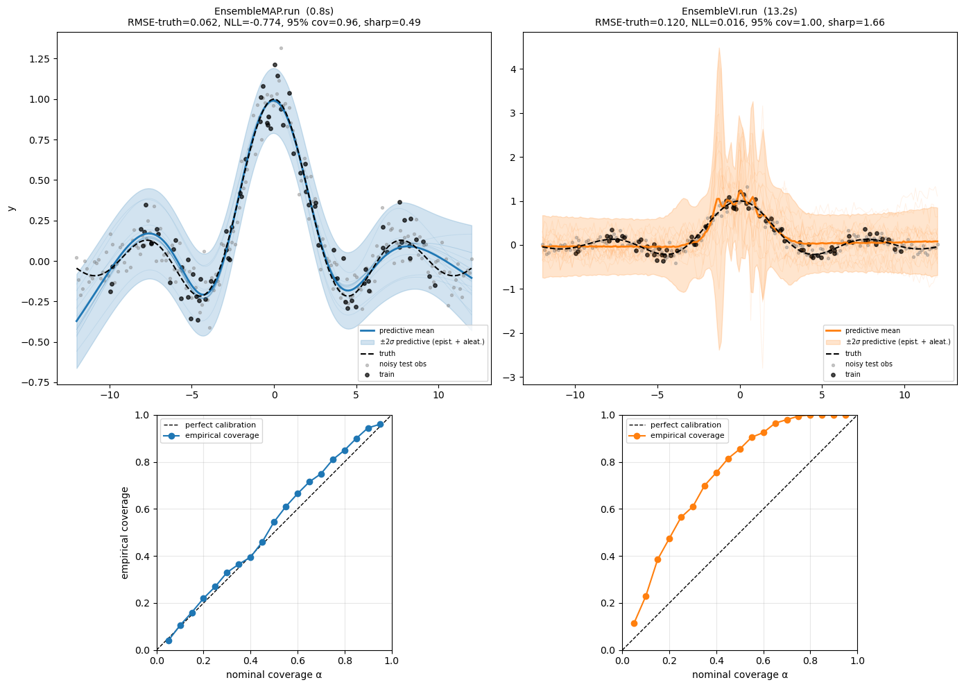
Summary table — full goodness-of-fit comparison¶

Takeaways¶

• Three call patterns, one object. init/update gives you full Python control; run gives you lax.scan speed; the bare ensemble_map function gives you a one-liner. Pick whichever ergonomics you need — the underlying maths is identical and init+update matches run to within seed-dependent permutation order.
• EnsembleMAP and EnsembleVI share an API. Same init / update / run triplet, same EnsembleResult(params, losses) return type. The only difference is what each member fits.
• MAP is near-oracle on this problem. All three MAP variants land at NLL $\approx -0.77$ against an oracle ceiling of -0.88, with 94% empirical coverage at the 95% nominal level and sharpness $\approx 0.41$ versus the irreducible $4\sigma = 0.40$. The point-mass mixture is doing essentially everything the data allows, and the predictive variance is dominated by aleatoric noise inside the training range.
• Mean-field VI is overdispersed here. With NLL $\approx 0$, 100% empirical coverage, and sharpness $\approx 1.7$ (more than $4\times$ the oracle), the VI ensemble buys coverage by paying a lot of sharpness — the bands are so wide they trivially contain every test observation, but the predictive density at any specific observation is small. This is the classic mean-field VI pathology: the diagonal-Gaussian factorization can’t represent the strong posterior correlations between MLP weights, so the posterior marginals end up much wider than they should be. Either a richer guide (low-rank, IAF, normalizing flow) or kl_weight < 1 (cold-posterior temper) typically helps.
• What “good” looks like. Read the calibration plots, NLL, and sharpness together. NLL alone catches both miscalibration and inaccuracy in one number; coverage tells you the direction of the miscalibration; sharpness tells you the price you’re paying for that coverage.
• When to drop down: if you need anything the runner doesn’t expose — custom batching, callbacks, early stopping, a non-standard inference loop — see the primitives tutorial.