Standard SVGP - Research Notebook

Standard SVGP with pyrox¶

The first notebook in the pyrox SVGP series: a textbook stochastic variational GP with $M$ inducing points living in the input space. Everything here is the reference that the next three notebooks will bend — notebook 2 trains the same model with mini-batches instead of full data, notebook 3 replaces the inducing points with a spherical-harmonic basis, notebook 4 warps the input space through a small neural network before the kernel sees it.

The goal for this notebook is narrow: set up the pyrox + optax scaffold that the later variants will reuse, and produce the canonical sanity-check plots — a monotone decreasing loss curve, inducing points migrating toward informative regions of the input, and a posterior mean + $2\sigma$ band that collapses onto the training data and widens over the input gap.

Background¶

Why sparse?¶

The exact GP posterior at $N$ training points and $N_*$ test points costs $\mathcal{O}(N^3)$ once and $\mathcal{O}(N^2 N_*)$ per prediction — the bottleneck being the solve against $K_{XX} + \sigma^2 I$ . With $N$ in the thousands this is already uncomfortable; with $N$ in the hundreds of thousands it is impossible on a single device. Sparse variational GPs (Titsias 2009, Hensman et al. 2013, 2015) replace the data-sized Gram matrix by a small $M \times M$ system over $M$ inducing values $u = f(Z)$ at user-chosen inducing inputs $Z \in \mathbb{R}^{M \times D}$ , with $M \ll N$ .

The ELBO¶

A variational posterior $q(u) = \mathcal{N}(m, S)$ induces a marginal Gaussian over the latent function at any input through the prior conditional $p(f \mid u)$ . The resulting variational lower bound on the log marginal likelihood is

\mathcal{L} = \sum_{n=1}^{N} \mathbb{E}_{q(f_n)}\!\bigl[\log p(y_n \mid f_n)\bigr] \;-\; \mathrm{KL}\!\bigl(q(u)\,\|\,p(u)\bigr),

(1)

with $p(u) = \mathcal{N}(0, K_{ZZ} + \text{jitter}\,I)$ . For Gaussian observation noise the expected log-likelihood has a closed form, so the ELBO is analytic and cheap to differentiate through — exactly the path pyrox.gp.svgp_elbo exposes.

The whitened parameterisation¶

Raw $q(u)$ couples the variational mean/covariance to the kernel through $K_{ZZ}$ — the loss landscape tilts as hyperparameters move. Hensman-et-al-2015 reparameterise in whitened coordinates $v$ with $u = L_{ZZ}\, v$ , $L_{ZZ} = \mathrm{chol}(K_{ZZ} + \text{jitter}\,I)$ , so the prior over $v$ is $\mathcal{N}(0, I)$ and the KL term decouples from the kernel. This is pyrox.gp.WhitenedGuide and it is the only guide that is both cheap and numerically robust for gradient-based training — we use it throughout the trilogy.

Setup¶

import equinox as eqx
import jax
import jax.numpy as jnp
import jax.random as jr
import matplotlib.pyplot as plt
import optax
from jaxtyping import Array, Float

from pyrox.gp import (
    GaussianLikelihood,
    Kernel,
    SparseGPPrior,
    WhitenedGuide,
    svgp_elbo,
)
from pyrox.gp._src.kernels import rbf_kernel

jax.config.update("jax_enable_x64", True)

/anaconda/lib/python3.13/site-packages/tqdm/auto.py:21: TqdmWarning: IProgress not found. Please update jupyter and ipywidgets. See https://ipywidgets.readthedocs.io/en/stable/user_install.html
  from .autonotebook import tqdm as notebook_tqdm

Toy data¶

A noisy 1-D sine with an extinction gap in the middle — $N = 500$ training points spread either side of the gap. The gap is the cheap sanity check: any well-fit GP should show a posterior band that narrows on the data and widens visibly where it has none.

key = jr.PRNGKey(0)
key, key_noise = jr.split(key)


def f_true(x: Float[Array, " N"]) -> Float[Array, " N"]:
    return jnp.sin(2.0 * x) + 0.3 * jnp.cos(5.0 * x)


N = 500
X_left = jr.uniform(jr.PRNGKey(1), (N // 2, 1), minval=-3.0, maxval=-0.6)
X_right = jr.uniform(jr.PRNGKey(2), (N // 2, 1), minval=0.6, maxval=3.0)
X_train = jnp.concatenate([X_left, X_right], axis=0)
noise_std = 0.15
y_train = f_true(X_train.squeeze(-1)) + noise_std * jr.normal(key_noise, (N,))
X_test = jnp.linspace(-3.5, 3.5, 400).reshape(-1, 1)

fig, ax = plt.subplots(figsize=(10, 3.5))
ax.scatter(X_train.squeeze(-1), y_train, s=8, alpha=0.4, label=f"training ($N={N}$)")
ax.plot(X_test.squeeze(-1), f_true(X_test.squeeze(-1)), "k--", lw=1.5, label="truth")
ax.set_xlabel("x")
ax.set_ylabel("y")
ax.set_title("Toy regression problem — noisy sine with an input gap")
ax.legend(loc="lower left")
plt.show()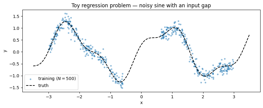

Kernel¶

The SVGP ELBO is a pure JAX function, so to train hyperparameters via optax we need the kernel to expose its scalars as equinox.Module array leaves — not hidden in the pyrox.Parameterized registry. Pattern A from exact_gp_regression.ipynb is the right tool: subclass the Kernel protocol with a plain equinox module and store unconstrained scalars on the log scale (so exp handles the positivity constraint for free).

class RBFLite(Kernel, eqx.Module):
    """Pure-equinox RBF — trainable log-variance / log-lengthscale scalars."""

    log_variance: Float[Array, ""]
    log_lengthscale: Float[Array, ""]

    @classmethod
    def init(cls, variance: float = 1.0, lengthscale: float = 1.0) -> "RBFLite":
        return cls(
            log_variance=jnp.log(jnp.asarray(variance)),
            log_lengthscale=jnp.log(jnp.asarray(lengthscale)),
        )

    @property
    def variance(self) -> Float[Array, ""]:
        return jnp.exp(self.log_variance)

    @property
    def lengthscale(self) -> Float[Array, ""]:
        return jnp.exp(self.log_lengthscale)

    def __call__(
        self,
        X1: Float[Array, "N1 D"],
        X2: Float[Array, "N2 D"],
    ) -> Float[Array, "N1 N2"]:
        return rbf_kernel(X1, X2, self.variance, self.lengthscale)

    def diag(self, X: Float[Array, "N D"]) -> Float[Array, " N"]:
        return self.variance * jnp.ones(X.shape[0], dtype=X.dtype)

The likelihood is GaussianLikelihood from pyrox — one field noise_var. Training noise_var directly would require a positivity projection; shipping a one-field wrapper that stores log_noise_var avoids the bookkeeping.

class TrainableGaussianLikelihood(eqx.Module):
    """Log-parameterised Gaussian likelihood; `.materialise()` returns the pyrox one."""

    log_noise_var: Float[Array, ""]

    @classmethod
    def init(cls, noise_var: float = 0.1) -> "TrainableGaussianLikelihood":
        return cls(log_noise_var=jnp.log(jnp.asarray(noise_var)))

    def materialise(self) -> GaussianLikelihood:
        return GaussianLikelihood(noise_var=jnp.exp(self.log_noise_var))

Model¶

$M = 20$ inducing points — placed by a Latin-style random sweep across the input range so they cover both data lobes and the gap. The gap locations will move toward the lobes during training; that migration is the headline visual of the notebook.

M = 20
key, key_z = jr.split(key)
Z_init = jr.uniform(key_z, (M, 1), minval=-3.0, maxval=3.0)

prior = SparseGPPrior(
    kernel=RBFLite.init(variance=1.0, lengthscale=0.6),
    Z=Z_init,
    jitter=1e-4,
)
guide = WhitenedGuide.init(num_inducing=M)
lik_w = TrainableGaussianLikelihood.init(noise_var=noise_std**2)

Training loop¶

svgp_elbo is a scalar JAX function of (prior, guide, lik, X, y) — put all three modules into a tuple, take eqx.filter_value_and_grad of the negative ELBO, and let optax.adam drive the leaves. Only array leaves get gradients; the rest of each module (the solver field, callbacks, etc.) is left alone.

Params = tuple  # alias: (prior, guide, lik_wrapper)


def neg_elbo(params: Params, X: Float[Array, "N D"], y: Float[Array, " N"]) -> Float[Array, ""]:
    prior_p, guide_p, lik_p = params
    lik = lik_p.materialise()
    return -svgp_elbo(prior_p, guide_p, lik, X, y)


@eqx.filter_jit
def step(
    params: Params,
    opt_state: optax.OptState,
    X: Float[Array, "N D"],
    y: Float[Array, " N"],
) -> tuple[Params, optax.OptState, Float[Array, ""]]:
    loss, grads = eqx.filter_value_and_grad(neg_elbo)(params, X, y)
    updates, opt_state = optimiser.update(grads, opt_state, params)
    params = eqx.apply_updates(params, updates)
    return params, opt_state, loss


params = (prior, guide, lik_w)
optimiser = optax.adam(5e-2)
opt_state = optimiser.init(eqx.filter(params, eqx.is_inexact_array))

Z_before = params[0].Z.copy()
n_steps = 800
losses: list[float] = []
for i in range(n_steps):
    params, opt_state, loss = step(params, opt_state, X_train, y_train)
    losses.append(float(loss))

prior_fit, guide_fit, lik_wrap_fit = params
Z_after = prior_fit.Z

print(f"final  -ELBO          = {losses[-1]:.3f}")
print(f"fitted variance       = {float(prior_fit.kernel.variance):.3f}")
print(f"fitted lengthscale    = {float(prior_fit.kernel.lengthscale):.3f}")
print(f"fitted noise std      = {float(jnp.exp(0.5 * lik_wrap_fit.log_noise_var)):.3f}  (truth {noise_std})")

final  -ELBO          = -193.226
fitted variance       = 0.559
fitted lengthscale    = 0.515
fitted noise std      = 0.154  (truth 0.15)

Loss curve¶

The first ~50 steps swallow almost all of the loss drop — the remaining 700 steps fine-tune kernel hyperparameters and inducing positions through a shallow tail. A symlog y-axis keeps both phases readable on one plot.

fig, ax = plt.subplots(figsize=(10, 3.5))
ax.plot(losses, color="C3", lw=1.5)
ax.set_xlabel("step")
ax.set_ylabel("−ELBO")
ax.set_yscale("symlog", linthresh=10.0)
ax.set_title("SVGP training — the negative ELBO we minimise")
ax.grid(alpha=0.3, which="both")
plt.show()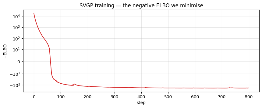

Inducing-point migration¶

Snapshot of the inducing inputs at step 0 (random initialisation) and at the end of training. A well-fit SVGP drags inducing points toward regions where they reduce the ELBO most — typically toward data-rich areas where the posterior wants sharp resolution. Expect the gap to be sparsely populated and the two data lobes to be denser.

A visible artefact. The ELBO penalises sloppy coverage but does not penalise two inducing points landing on top of each other — the KL term handles that degeneracy silently via a correlated q(u). You’ll often see small pile-ups (e.g. two points coincident around x ≈ 1.4 in the fitted row below). Fixing it properly takes either a repulsive regulariser on Z or a different inducing parameterisation — exactly the door that notebook 3 opens with spherical-harmonic features, where “inducing points” become a fixed orthogonal basis and the pile-up failure mode can’t exist.

fig, ax = plt.subplots(figsize=(10, 2.6))
ax.scatter(X_train.squeeze(-1), jnp.full_like(X_train.squeeze(-1), 0.2), s=5, alpha=0.3, color="gray", label="training x")
ax.scatter(Z_before.squeeze(-1), jnp.full((M,), 0.5), s=60, marker="x", color="C0", label="Z init", zorder=4)
ax.scatter(Z_after.squeeze(-1), jnp.full((M,), 0.8), s=60, marker="o", facecolors="none", edgecolors="C3", linewidths=1.8, label="Z after fit", zorder=5)
ax.set_yticks([0.2, 0.5, 0.8])
ax.set_yticklabels(["data", "init", "fitted"])
ax.set_xlabel("x")
ax.set_xlim(-3.5, 3.5)
ax.set_ylim(0, 1.0)
ax.set_title("Inducing-point migration during SVGP training")
ax.legend(loc="upper right", fontsize=9)
plt.show()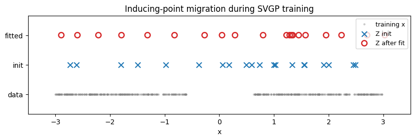

Posterior predictive¶

pyrox.gp.WhitenedGuide.predict(K_xz, K_zz_op, K_xx_diag) returns posterior mean and variance at any test set given the three predictive blocks from the sparse prior. Add the prior’s mean function (zero here) back on, then overlay the $\pm 2\sigma$ band on top of the training scatter.

K_zz_op, K_xz, K_xx_diag = prior_fit.predictive_blocks(X_test)
f_loc, f_var = guide_fit.predict(K_xz, K_zz_op, K_xx_diag)
f_loc = f_loc + prior_fit.mean(X_test)
noise_var_fit = jnp.exp(lik_wrap_fit.log_noise_var)
y_std = jnp.sqrt(f_var + noise_var_fit)

fig, ax = plt.subplots(figsize=(10, 4.0))
ax.fill_between(
    X_test.squeeze(-1),
    f_loc - 2 * y_std,
    f_loc + 2 * y_std,
    alpha=0.25,
    color="C0",
    label=r"$\pm 2\sigma$ (predictive)",
)
ax.plot(X_test.squeeze(-1), f_loc, "C0-", lw=2, label="posterior mean")
ax.plot(X_test.squeeze(-1), f_true(X_test.squeeze(-1)), "k--", lw=1.2, label="truth")
ax.scatter(X_train.squeeze(-1), y_train, s=6, alpha=0.35, color="gray", label="training")
ax.scatter(
    Z_after.squeeze(-1),
    jnp.full((M,), ax.get_ylim()[0] + 0.05),
    s=50,
    marker="|",
    color="C3",
    label="inducing inputs",
)
ax.set_xlabel("x")
ax.set_ylabel("y")
ax.set_title("SVGP posterior — mean + $2\\sigma$ predictive band")
ax.legend(loc="lower left", fontsize=9)
plt.show()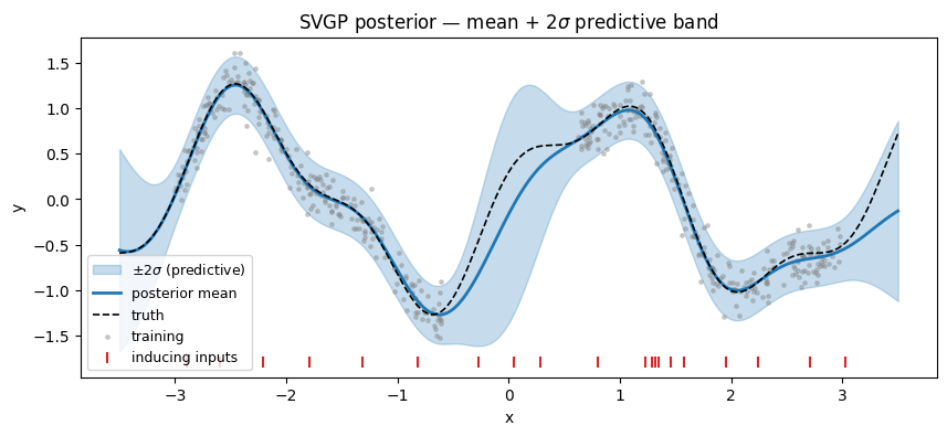

A note on the gap. The posterior mean is smoother across the input gap than the truth (the true function has a local min near x ≈ -0.3 that the blue mean rounds off). This is not a bug — with only $M = 20$ inducing points and a lengthscale fit at $\ell \approx 0.5$ against a gap about 1.2 units wide, the model has no data and limited inducing density there, so the posterior relaxes toward the prior (zero-mean, wide band). Widening the band is the epistemically correct response; getting the mean exactly right over the gap would require either more inducing capacity or a stronger structural prior (e.g. periodic kernel).

Summary¶

SparseGPPrior(kernel, Z) + WhitenedGuide + GaussianLikelihood is the canonical SVGP triple.
svgp_elbo is a pure JAX scalar so optax + eqx.filter_value_and_grad trains everything jointly (kernel hyperparameters, inducing inputs, guide parameters, noise).
The fitted lengthscale and noise should be close to the true generating values; inducing points migrate toward data lobes.

Next: notebook 2 keeps this exact model but swaps the full-data ELBO for an unbiased mini-batch estimator — the main reason you’d reach for SVGP instead of an exact GP in the first place.