Batched SVGP - Research Notebook

Batched SVGP — the main reason you’d use one¶

The first notebook in this series built the standard SVGP scaffold on $N = 500$ observations. That’s small enough that every optimiser step used the full dataset. The whole point of SVGP, though, is to scale — and the mechanism is mini-batch training against an unbiased ELBO estimator.

This notebook stays inside the exact same pyrox + optax scaffold as notebook 1, flips one switch — replace the full dataset in each gradient step with a randomly sampled mini-batch — and shows the consequence on wallclock, convergence, and the final posterior.

Why SVGP mini-batches at all¶

The ELBO decomposes additively over data¶

Every SVGP ELBO (Gaussian or otherwise) has the structure

\mathcal{L} = \underbrace{\sum_{n=1}^{N} \mathbb{E}_{q(f_n)}\!\bigl[\log p(y_n \mid f_n)\bigr]}_{\text{ELL — sum over data}} \;-\; \underbrace{\mathrm{KL}\bigl(q(u) \;\|\; p(u)\bigr)}_{\text{fixed, cost } \mathcal{O}(M^3)}.

(1)

The first term is a sum over independent data points. So if we pick a uniform random subset $\mathcal{B} \subset \{1, \dots, N\}$ of size $B$ , then the unbiased mini-batch ELBO is

\tilde{\mathcal{L}}(\mathcal{B}) = \frac{N}{B}\sum_{n \in \mathcal{B}} \mathbb{E}_{q(f_n)}\!\bigl[\log p(y_n \mid f_n)\bigr] \;-\; \mathrm{KL}\bigl(q(u) \;\|\; p(u)\bigr),

(2)

with $\mathbb{E}_\mathcal{B}[\tilde{\mathcal{L}}] = \mathcal{L}$ . Stochastic gradients of $\tilde{\mathcal{L}}$ are unbiased estimates of the gradients of $\mathcal{L}$ , and optax.adam handles the variance.

Cost per step¶

For a single SVGP ELBO evaluation, the dominant terms are

$\mathcal{O}(B M^2)$ for the cross-covariance $K_{xZ}$ and the predictive contraction.
$\mathcal{O}(M^3)$ for the inducing-prior Cholesky (shared across all batches in a step, not scaling with $B$ ).

Full-batch cost is $\mathcal{O}(N M^2 + M^3)$ . Mini-batch cost is $\mathcal{O}(B M^2 + M^3)$ . Once $N \gg B$ the speedup approaches $N / B$ — the point of the exercise.

What doesn’t change¶

The KL term, the inducing inputs, the variational Cholesky — they all sit on the “model side” of the ELBO and are identical to the full-batch version. The only bookkeeping is (i) scale the ELL by $N / B$ , (ii) sample a different batch each step.

Setup¶

import time

import equinox as eqx
import jax
import jax.numpy as jnp
import jax.random as jr
import matplotlib.pyplot as plt
import optax
from jaxtyping import Array, Float

from pyrox.gp import (
    GaussianLikelihood,
    Kernel,
    SparseGPPrior,
    WhitenedGuide,
    svgp_elbo,
)
from pyrox.gp._src.kernels import rbf_kernel

jax.config.update("jax_enable_x64", True)

/anaconda/lib/python3.13/site-packages/tqdm/auto.py:21: TqdmWarning: IProgress not found. Please update jupyter and ipywidgets. See https://ipywidgets.readthedocs.io/en/stable/user_install.html
  from .autonotebook import tqdm as notebook_tqdm

A bigger dataset¶

$N = 10\,000$ points drawn from a 2-D function with a sharp central feature and smoother tails — enough data that full-batch gradient steps start to feel sluggish, but small enough that we can still run the full-batch baseline as a correctness check.

def f_true(X: Float[Array, "N 2"]) -> Float[Array, " N"]:
    r2 = X[:, 0] ** 2 + X[:, 1] ** 2
    return jnp.sin(3.0 * X[:, 0]) * jnp.exp(-1.5 * r2) + 0.3 * X[:, 1]


key = jr.PRNGKey(0)
key, key_X, key_noise = jr.split(key, 3)
N = 10_000
X_train = jr.uniform(key_X, (N, 2), minval=-1.5, maxval=1.5)
noise_std = 0.1
y_train = f_true(X_train) + noise_std * jr.normal(key_noise, (N,))

# Evaluation grid for posterior comparison
G = 60
g = jnp.linspace(-1.5, 1.5, G)
X1g, X2g = jnp.meshgrid(g, g, indexing="xy")
X_grid = jnp.stack([X1g.ravel(), X2g.ravel()], axis=-1)
y_grid_true = f_true(X_grid).reshape(G, G)

fig, ax = plt.subplots(figsize=(5.5, 4.5))
mesh = ax.pcolormesh(X1g, X2g, y_grid_true, cmap="RdBu_r", vmin=-0.8, vmax=0.8, shading="auto")
ax.scatter(X_train[::50, 0], X_train[::50, 1], s=1.5, alpha=0.25, color="k")
fig.colorbar(mesh, ax=ax, label="f(x)")
ax.set_xlabel("$x_1$")
ax.set_ylabel("$x_2$")
ax.set_aspect("equal")
ax.set_title(f"Target function — $N = {N:,}$ training points (every 50th shown)")
plt.show()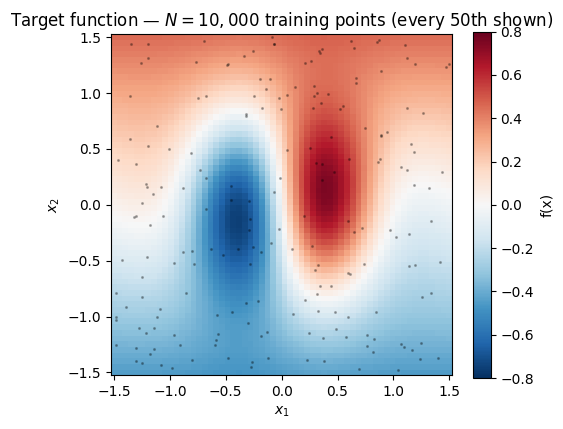

Kernel + likelihood + guide¶

Same RBFLite pattern from notebook 1 and a TrainableGaussianLikelihood wrapper so the noise variance stays positive during optimisation. $M = 50$ inducing points on a $10 \times 5$ grid.

class RBFLite(Kernel, eqx.Module):
    log_variance: Float[Array, ""]
    log_lengthscale: Float[Array, ""]

    @classmethod
    def init(cls, variance: float = 1.0, lengthscale: float = 1.0) -> "RBFLite":
        return cls(
            log_variance=jnp.log(jnp.asarray(variance)),
            log_lengthscale=jnp.log(jnp.asarray(lengthscale)),
        )

    @property
    def variance(self) -> Float[Array, ""]:
        return jnp.exp(self.log_variance)

    @property
    def lengthscale(self) -> Float[Array, ""]:
        return jnp.exp(self.log_lengthscale)

    def __call__(self, X1, X2):
        return rbf_kernel(X1, X2, self.variance, self.lengthscale)

    def diag(self, X):
        return self.variance * jnp.ones(X.shape[0], dtype=X.dtype)


class TrainableGaussianLikelihood(eqx.Module):
    log_noise_var: Float[Array, ""]

    @classmethod
    def init(cls, noise_var: float = 0.1) -> "TrainableGaussianLikelihood":
        return cls(log_noise_var=jnp.log(jnp.asarray(noise_var)))

    def materialise(self) -> GaussianLikelihood:
        return GaussianLikelihood(noise_var=jnp.exp(self.log_noise_var))


M = 50
gx, gy = jnp.meshgrid(jnp.linspace(-1.3, 1.3, 10), jnp.linspace(-1.3, 1.3, 5), indexing="xy")
Z_init = jnp.stack([gx.ravel(), gy.ravel()], axis=-1)


def fresh_model() -> tuple:
    return (
        SparseGPPrior(
            kernel=RBFLite.init(variance=1.0, lengthscale=0.5),
            Z=Z_init,
            jitter=1e-4,
        ),
        WhitenedGuide.init(num_inducing=M),
        TrainableGaussianLikelihood.init(noise_var=noise_std**2),
    )

The mini-batch ELBO — scale the ELL, not the KL¶

pyrox.gp.svgp_elbo returns ELL_batch − KL. To turn that into an unbiased estimator of the full-data ELBO from a batch of size $B$ , multiply the ELL by $N/B$ but leave the KL alone. Algebra:

\tilde{\mathcal{L}} = \frac{N}{B}\,\mathrm{ELL}_{\mathcal{B}} - \mathrm{KL} = \frac{N}{B}\bigl(\text{svgp\_elbo}_{\mathcal{B}} + \mathrm{KL}\bigr) - \mathrm{KL} = \frac{N}{B}\,\text{svgp\_elbo}_{\mathcal{B}} + \Bigl(\frac{N}{B} - 1\Bigr)\mathrm{KL}.

(3)

The KL is exposed on guide.kl_divergence(K_zz_op), so we can recover it independently.

def scaled_neg_elbo(
    params: tuple,
    X_batch: Float[Array, "B 2"],
    y_batch: Float[Array, " B"],
    N_total: int,
) -> Float[Array, ""]:
    prior, guide, lik_w = params
    lik = lik_w.materialise()
    elbo_batch = svgp_elbo(prior, guide, lik, X_batch, y_batch)
    K_zz_op = prior.inducing_operator()
    kl = guide.kl_divergence(K_zz_op)  # ty: ignore[unresolved-attribute]
    B = X_batch.shape[0]
    scale = N_total / B
    return -(scale * elbo_batch + (scale - 1.0) * kl)

Baseline — full-batch training¶

We JIT a step, spin for n_steps_full = 300 and record wallclock.

n_steps_full = 300
lr = 5e-2


def train_full_batch(X: Float[Array, "N 2"], y: Float[Array, " N"]) -> tuple:
    params = fresh_model()
    optimiser = optax.adam(lr)
    opt_state = optimiser.init(eqx.filter(params, eqx.is_inexact_array))

    @eqx.filter_jit
    def step(params, opt_state):
        loss, grads = eqx.filter_value_and_grad(scaled_neg_elbo)(params, X, y, X.shape[0])
        updates, opt_state = optimiser.update(grads, opt_state, params)
        return eqx.apply_updates(params, updates), opt_state, loss

    # warmup compile
    step(params, opt_state)[2].block_until_ready()
    losses = []
    t0 = time.time()
    for _ in range(n_steps_full):
        params, opt_state, loss = step(params, opt_state)
        losses.append(float(loss))
    wall = time.time() - t0
    return params, losses, wall


params_full, losses_full, wall_full = train_full_batch(X_train, y_train)
print(f"full batch ({N:,} pts)   |  {n_steps_full} steps  |  {wall_full:.2f} s  |"
      f"  {wall_full / n_steps_full * 1000:.1f} ms/step")

full batch (10,000 pts)   |  300 steps  |  15.31 s  |  51.0 ms/step

Mini-batch training¶

Sample a fixed-size batch of indices per step via jr.randint (with replacement — statistically almost identical to without-replacement for $B \ll N$ and avoids a dynamic choice that would recompile). B = 200 — 50× smaller than $N$ , should give a comparable per-step speedup.

B = 200
n_steps_mini = 300 * 50  # match total data throughput approximately


def train_minibatch(X: Float[Array, "N 2"], y: Float[Array, " N"]) -> tuple:
    N_total = X.shape[0]
    params = fresh_model()
    optimiser = optax.adam(lr)
    opt_state = optimiser.init(eqx.filter(params, eqx.is_inexact_array))

    @eqx.filter_jit
    def step(params, opt_state, key):
        idx = jr.randint(key, (B,), 0, N_total)
        X_b = X[idx]
        y_b = y[idx]
        loss, grads = eqx.filter_value_and_grad(scaled_neg_elbo)(params, X_b, y_b, N_total)
        updates, opt_state = optimiser.update(grads, opt_state, params)
        return eqx.apply_updates(params, updates), opt_state, loss

    key_base = jr.PRNGKey(17)
    keys = jr.split(key_base, n_steps_mini)
    # warmup
    step(params, opt_state, keys[0])[2].block_until_ready()
    losses = []
    t0 = time.time()
    for k in keys:
        params, opt_state, loss = step(params, opt_state, k)
        losses.append(float(loss))
    wall = time.time() - t0
    return params, losses, wall


params_mini, losses_mini, wall_mini = train_minibatch(X_train, y_train)
print(f"mini-batch ({B} pts)    |  {n_steps_mini} steps  |  {wall_mini:.2f} s  |"
      f"  {wall_mini / n_steps_mini * 1000:.2f} ms/step")

mini-batch (200 pts)    |  15000 steps  |  60.04 s  |  4.00 ms/step

Per-step speedup¶

A single mini-batch step should be much faster than a full-batch step. At $B = 200$ and $N = 10\,000$ the theoretical cost ratio is ~50×; actual hardware behaviour depends on whether the GPU is memory-bound or compute-bound at these sizes.

speedup = (wall_full / n_steps_full) / (wall_mini / n_steps_mini)
print(f"per-step speedup:  {speedup:.1f}×   (theoretical ceiling ≈ {N / B}×)")

per-step speedup:  12.8×   (theoretical ceiling ≈ 50.0×)

Convergence curves¶

Plot loss vs wallclock, not step — step is the wrong axis for this comparison. Mini-batch does many more steps than full-batch in the same wallclock budget, which is exactly the point.

def to_wallclock(losses: list[float], wall: float) -> Float[Array, " n"]:
    return jnp.linspace(0.0, wall, len(losses))


fig, axes = plt.subplots(1, 2, figsize=(13, 4.2))
ax = axes[0]
ax.plot(to_wallclock(losses_full, wall_full), losses_full, color="C0", lw=1.4, label=f"full batch (N = {N:,})")
ax.plot(to_wallclock(losses_mini, wall_mini), losses_mini, color="C3", lw=0.9, alpha=0.8, label=f"mini-batch (B = {B})")
ax.set_xlabel("wallclock [s]")
ax.set_ylabel("−ELBO")
ax.set_yscale("symlog", linthresh=100.0)
ax.set_title("Convergence vs wallclock")
ax.legend()
ax.grid(alpha=0.3, which="both")

ax = axes[1]
ax.plot(losses_full, color="C0", lw=1.4, label="full batch")
ax.plot(losses_mini, color="C3", lw=0.8, alpha=0.7, label="mini-batch")
ax.set_xlabel("step")
ax.set_ylabel("−ELBO")
ax.set_yscale("symlog", linthresh=100.0)
ax.set_title("Convergence vs step (different meaning per curve)")
ax.legend()
ax.grid(alpha=0.3, which="both")
plt.tight_layout()
plt.show()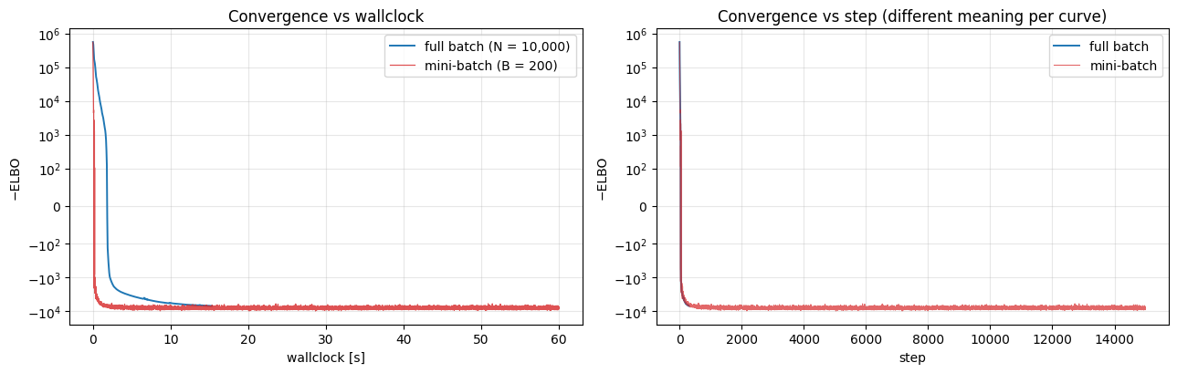

The left panel is the honest comparison. The right is the illusion: the mini-batch curve looks noisier per “step” because each step uses 50× less data, so the stochastic gradient has ~ $\sqrt{50}$ × more variance. The stochasticity is a feature of the estimator, not a fit quality problem — the optimiser still converges in expectation.

Posterior agreement¶

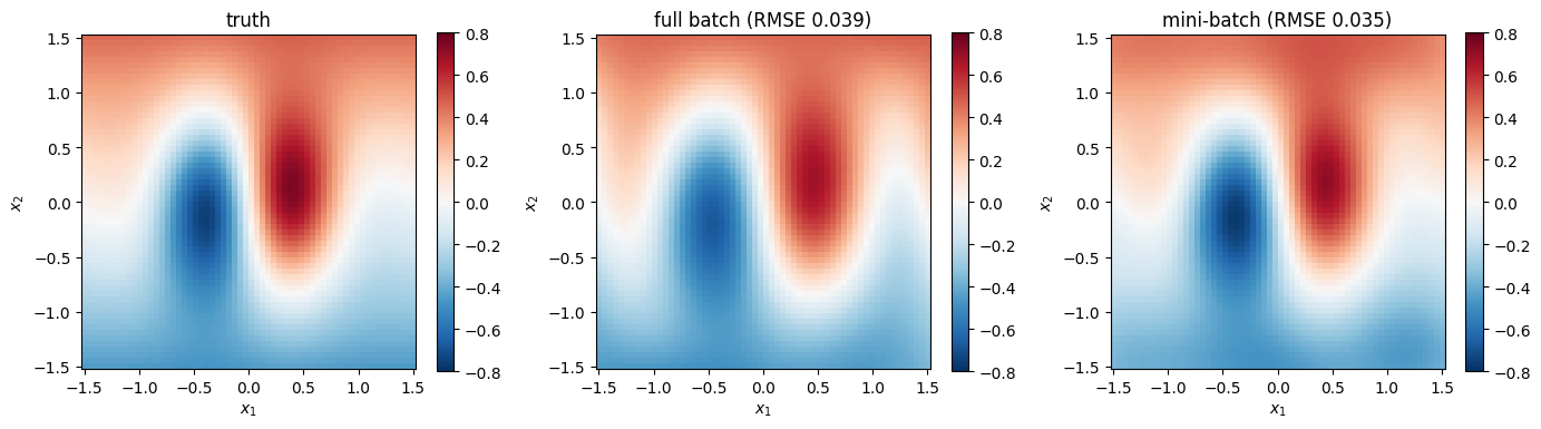
Full and mini-batch should arrive at the same posterior (up to stochastic noise and the extra training steps). Evaluate both on the $60 \times 60$ grid and map.

def posterior_mean(params, X_eval):
    prior_fit, guide_fit, _ = params
    K_zz_op, K_xz, K_xx_diag = prior_fit.predictive_blocks(X_eval)
    f_loc, _ = guide_fit.predict(K_xz, K_zz_op, K_xx_diag)
    return (f_loc + prior_fit.mean(X_eval)).reshape(G, G)


mean_full = posterior_mean(params_full, X_grid)
mean_mini = posterior_mean(params_mini, X_grid)

rmse_full = float(jnp.sqrt(jnp.mean((mean_full - y_grid_true) ** 2)))
rmse_mini = float(jnp.sqrt(jnp.mean((mean_mini - y_grid_true) ** 2)))
rmse_disagreement = float(jnp.sqrt(jnp.mean((mean_full - mean_mini) ** 2)))
print(f"grid RMSE vs truth — full batch : {rmse_full:.4f}")
print(f"grid RMSE vs truth — mini-batch : {rmse_mini:.4f}")
print(f"grid RMSE mini ↔ full disagreement: {rmse_disagreement:.4f}")

fig, axes = plt.subplots(1, 3, figsize=(14, 4.2))
for ax, field, title in zip(
    axes,
    [y_grid_true, mean_full, mean_mini],
    ["truth", f"full batch (RMSE {rmse_full:.3f})", f"mini-batch (RMSE {rmse_mini:.3f})"],
    strict=True,
):
    mesh = ax.pcolormesh(X1g, X2g, field, cmap="RdBu_r", vmin=-0.8, vmax=0.8, shading="auto")
    fig.colorbar(mesh, ax=ax, shrink=0.8)
    ax.set_aspect("equal")
    ax.set_xlabel("$x_1$")
    ax.set_ylabel("$x_2$")
    ax.set_title(title)
plt.tight_layout()
plt.show()

grid RMSE vs truth — full batch : 0.0386
grid RMSE vs truth — mini-batch : 0.0350
grid RMSE mini ↔ full disagreement: 0.0446

Batch-size sweep — where does the speedup saturate?¶

A common practical question: if $B = 200$ gives a $\sim 50\times$ per-step speedup, does $B = 20$ give $500\times$ ? Answer in general: no — GPU dispatch overhead dominates below a certain batch size, so there’s a regime where smaller batches don’t help. Timing sweep below.

def time_one_step(B_try: int, n_warmup: int = 3, n_time: int = 30) -> float:
    params = fresh_model()
    optimiser = optax.adam(lr)
    opt_state = optimiser.init(eqx.filter(params, eqx.is_inexact_array))

    @eqx.filter_jit
    def step(params, opt_state, idx):
        X_b = X_train[idx]
        y_b = y_train[idx]
        loss, grads = eqx.filter_value_and_grad(scaled_neg_elbo)(params, X_b, y_b, N)
        updates, opt_state = optimiser.update(grads, opt_state, params)
        return eqx.apply_updates(params, updates), opt_state, loss

    key_s = jr.split(jr.PRNGKey(0), n_warmup + n_time)
    idx_arrs = [jr.randint(k, (B_try,), 0, N) for k in key_s]
    for i in range(n_warmup):
        params, opt_state, _ = step(params, opt_state, idx_arrs[i])
    t0 = time.time()
    for i in range(n_warmup, n_warmup + n_time):
        params, opt_state, _ = step(params, opt_state, idx_arrs[i])
    # Force the last compute to complete.
    params[0].inducing_operator().as_matrix().block_until_ready()
    return (time.time() - t0) / n_time * 1000  # ms per step


Bs = [32, 64, 128, 256, 512, 1024, 2048, 5000, N]
ms_per_step = [time_one_step(B_) for B_ in Bs]
for B_, t in zip(Bs, ms_per_step, strict=True):
    tag = " (= N)" if B_ == N else ""
    print(f"B = {B_:>5}{tag}   {t:6.2f} ms/step")

B =    32     1.94 ms/step
B =    64     1.74 ms/step
B =   128     3.82 ms/step
B =   256    31.44 ms/step
B =   512    18.52 ms/step
B =  1024    35.41 ms/step
B =  2048    39.59 ms/step
B =  5000    45.52 ms/step
B = 10000 (= N)    67.47 ms/step

fig, ax = plt.subplots(figsize=(8, 4))
ax.loglog(Bs, ms_per_step, "o-", color="C3", lw=1.8)
ax.set_xlabel("batch size B")
ax.set_ylabel("ms / step")
ax.set_title("SVGP step cost vs batch size")
ax.grid(alpha=0.3, which="both")
# Mark the full-batch point
ax.axvline(N, color="k", ls="--", alpha=0.4, label=f"full batch (B = N = {N:,})")
ax.legend()
plt.show()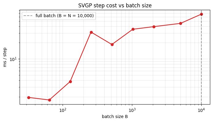

Two readable regimes: a flat region at small $B$ where per-step cost is dominated by kernel/guide overhead and the $\mathcal{O}(M^3)$ inducing Cholesky, and a rising region where $\mathcal{O}(B M^2)$ starts to matter and the curve approaches the full-batch cost. The inflection sits around $B \approx 500$ at $M = 50$ on this hardware; the right batch size is “a bit smaller than the inflection” — enough to amortise the overhead but not so large that you’re paying the full-batch rate.

Summary¶

pyrox.gp.svgp_elbo is a pure JAX function of (prior, guide, lik, X, y) — hand it a batch instead of the whole dataset, rescale the ELL by $N/B$ , and you have an unbiased ELBO estimator.
The KL term is computed separately from guide.kl_divergence(K_zz_op) so it can be held out of the ELL rescaling — the clean decomposition is ÑL̂ = (N/B) · svgp_elbo_batch + (N/B − 1) · KL.
Per-step wallclock drops roughly proportionally to $B/N$ until GPU dispatch overhead takes over at small $B$ . The sweet spot sits an order of magnitude below the inflection point of that curve.
Mini-batch SGD arrives at the same posterior as full-batch training to within stochastic noise — the noisier loss curve is not a fit quality problem.

Next: notebook 3 keeps the point-inducing + whitened-guide scaffold but replaces $Z \in \mathbb{R}^{M \times D}$ with a fixed spherical-harmonic basis, collapsing the $\mathcal{O}(M^3)$ inducing Cholesky to $\mathcal{O}(M)$ .