EVT Distributions: A Visual & Physical Tour

This notebook is a gallery of the five extreme-value distributions exposed by xtremax.distributions. For each one we plot the PDF and CDF over a small parameter sweep, draw a sample and overlay the analytic density, and show a return-level curve. The narrative cells say what the distribution is, how the parameters move it around, and which physical phenomena it tends to fit.

Distributions covered

Class	Family	Shape ξ	Tail behaviour
`GumbelType1GEVD`	GEVD Type I	ξ = 0	Exponential, unbounded
`FrechetType2GEVD`	GEVD Type II	ξ > 0	Heavy polynomial, lower-bounded
`WeibullType3GEVD`	GEVD Type III	ξ < 0	Light, upper-bounded
`GeneralizedExtremeValueDistribution`	GEVD (general)	ξ ∈ ℝ	All three regimes
`GeneralizedParetoDistribution`	GPD (POT)	ξ ∈ ℝ	Excesses over a threshold

Why these five? The Fisher–Tippett–Gnedenko theorem states that the only non-degenerate limits for normalised block maxima of i.i.d. samples are the three GEVD types. The Pickands–Balkema–de Haan theorem gives the parallel statement for threshold exceedances: their limit law is the GPD. Together they are the canonical building blocks of classical extreme-value theory.

import subprocess
import sys


try:
    import google.colab  # noqa: F401

    IN_COLAB = True
except ImportError:
    IN_COLAB = False

if IN_COLAB:
    subprocess.run(
        [
            sys.executable,
            "-m",
            "pip",
            "install",
            "-q",
            "xtremax @ git+https://github.com/jejjohnson/xtremax@main",
        ],
        check=True,
    )

import warnings


warnings.filterwarnings("ignore", message=r".*IProgress.*")

import jax
import jax.numpy as jnp
import matplotlib.pyplot as plt
import numpy as np

from xtremax.distributions import (
    FrechetType2GEVD,
    GeneralizedExtremeValueDistribution,
    GeneralizedParetoDistribution,
    GumbelType1GEVD,
    WeibullType3GEVD,
)


KEY = jax.random.PRNGKey(0)

import importlib.util


try:
    from IPython import get_ipython

    ipython = get_ipython()
except ImportError:
    ipython = None

if ipython is not None and importlib.util.find_spec("watermark") is not None:
    ipython.run_line_magic("load_ext", "watermark")
    ipython.run_line_magic(
        "watermark",
        "-v -m -p jax,numpy,matplotlib,numpyro,xtremax",
    )
else:
    print("watermark extension not loaded (IPython or watermark package missing)")

Python implementation: CPython
Python version       : 3.13.5
IPython version      : 9.10.0

jax       : 0.6.2
numpy     : 2.4.4
matplotlib: 3.10.8
numpyro   : 0.19.0
xtremax   : 0.0.0

Compiler    : GCC 11.2.0
OS          : Linux
Release     : 6.8.0-1044-azure
Machine     : x86_64
Processor   : x86_64
CPU cores   : 16
Architecture: 64bit

A unified parameterisation¶

All three GEVD types share a single Coles (2001) parameterisation

F(x;\,\mu,\sigma,\xi) \;=\; \begin{cases} \exp\!\left\{-\bigl[1 + \xi\,\tfrac{x-\mu}{\sigma}\bigr]^{-1/\xi}\right\}, & \xi \neq 0,\\[6pt] \exp\!\left\{-\exp\!\bigl(-\tfrac{x-\mu}{\sigma}\bigr)\right\}, & \xi = 0, \end{cases}

(1)

with $\sigma > 0$ and support determined by $1 + \xi(x - \mu)/\sigma > 0$ . Differentiating gives the PDF

f(x) = \frac{1}{\sigma}\bigl[1 + \xi\,\tfrac{x-\mu}{\sigma}\bigr]^{-(1/\xi + 1)} \,\exp\!\left\{-\bigl[1 + \xi\,\tfrac{x-\mu}{\sigma}\bigr]^{-1/\xi}\right\},\quad \xi \neq 0.

(2)

The three classical types are slices of this family at $\xi=0$ (Gumbel), $\xi>0$ (Fréchet) and $\xi<0$ (Weibull). The GPD has an analogous structure for excesses $y = x - u$ over a threshold $u$ :

F_{\text{GPD}}(y;\,\sigma,\xi) = \begin{cases} 1 - \bigl[1 + \xi\,\tfrac{y}{\sigma}\bigr]^{-1/\xi}, & \xi \neq 0,\\[6pt] 1 - \exp(-y/\sigma), & \xi = 0, \end{cases}

(3)

defined on $y \ge 0$ (and $y \le -\sigma/\xi$ if $\xi < 0$ ). The GPD shape parameter $\xi$ is the same one that appears in the GEVD limit of the parent distribution: this is the Pickands–Balkema–de Haan theorem.

In the cells below we share a small helper that draws PDF, CDF and a histogram-vs-density panel for whichever distribution we hand it.

def plot_pdf_cdf(
    dist_factory,
    param_grid,
    label_fn,
    title,
    x_range,
    n_grid=400,
    sample_size=20_000,
    key=None,
):
    """Plot PDF, CDF and a histogram-vs-density panel for a parameter sweep.

    `dist_factory(**params)` constructs a distribution from a row of `param_grid`.
    `label_fn(params)` returns the legend label for that row.
    """
    if key is None:
        key = jax.random.PRNGKey(1)
    xs = jnp.linspace(*x_range, n_grid)
    fig, axes = plt.subplots(1, 3, figsize=(16, 4.2))
    keys = jax.random.split(key, len(param_grid))
    for _k, params in zip(keys, param_grid, strict=True):
        d = dist_factory(**params)
        log_pdf = d.log_prob(xs)
        cdf = d.cdf(xs)
        axes[0].plot(xs, jnp.exp(log_pdf), label=label_fn(params))
        axes[1].plot(xs, cdf, label=label_fn(params))
    sample_params = param_grid[len(param_grid) // 2]
    d = dist_factory(**sample_params)
    samples = np.asarray(d.sample(keys[0], (sample_size,)))
    finite = samples[np.isfinite(samples)]
    axes[2].hist(
        finite,
        bins=80,
        range=x_range,
        density=True,
        alpha=0.45,
        color="tab:gray",
        label="samples",
    )
    axes[2].plot(
        xs,
        jnp.exp(d.log_prob(xs)),
        color="tab:red",
        lw=2,
        label=f"PDF, {label_fn(sample_params)}",
    )
    for ax in axes:
        ax.grid(True, alpha=0.3)
        ax.set_xlabel("x")
    axes[0].set_ylabel("f(x)")
    axes[0].set_title("PDF")
    axes[1].set_ylabel("F(x)")
    axes[1].set_title("CDF")
    axes[2].set_ylabel("density")
    axes[2].set_title("Sample vs PDF")
    for ax in axes:
        ax.legend(fontsize=8)
    fig.suptitle(title, y=1.02)
    plt.tight_layout()
    plt.show()
    return fig


def plot_return_levels(
    dist_factory,
    param_grid,
    label_fn,
    title,
    periods=None,
):
    """Return level vs return period (log-x) for a parameter sweep."""
    if periods is None:
        periods = jnp.logspace(0.1, 3, 80)
    fig, ax = plt.subplots(figsize=(8, 4.5))
    for params in param_grid:
        d = dist_factory(**params)
        rl = d.return_level(periods)
        ax.plot(periods, rl, label=label_fn(params))
    ax.set_xscale("log")
    ax.set_xlabel("Return period T (blocks)")
    ax.set_ylabel("Return level $z_T$")
    ax.set_title(title)
    ax.grid(True, which="both", alpha=0.3)
    ax.legend(fontsize=9)
    plt.tight_layout()
    plt.show()
    return fig

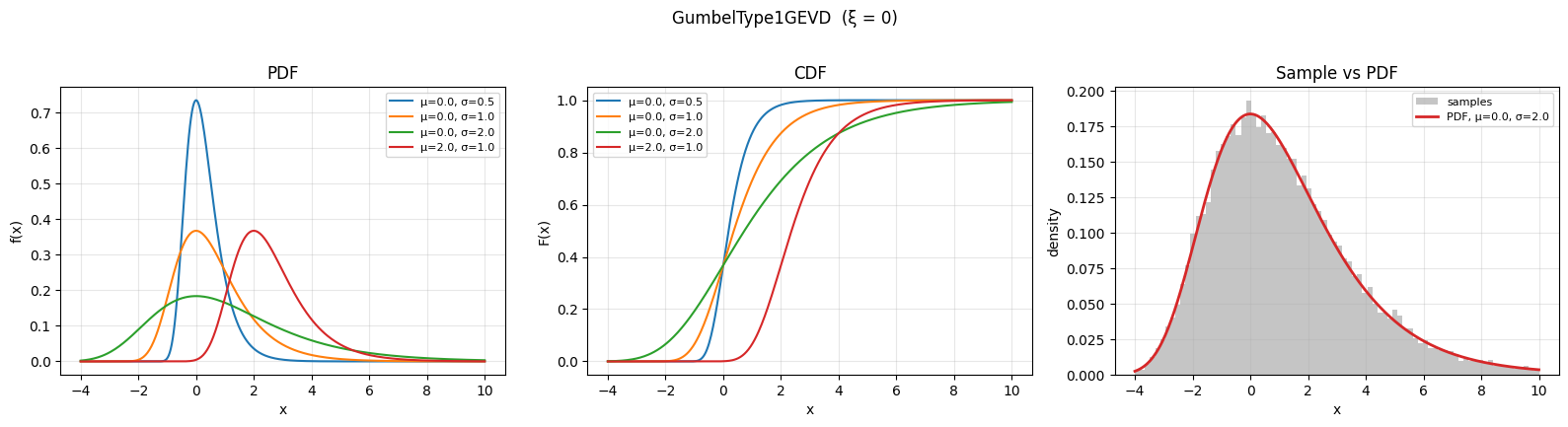
1. Gumbel (Type I, ξ = 0)¶

The Gumbel is the GEVD limit when the parent distribution has exponentially decaying tails (e.g. Gaussian, exponential, gamma). It has unbounded support, finite moments of every order, and a fixed positive skewness $\approx 1.14$ .

Density and CDF (with standardised variate $z = (x-\mu)/\sigma$ ):

f(x) = \tfrac{1}{\sigma}\,e^{-z}\,\exp(-e^{-z}),\qquad F(x) = \exp(-e^{-z}).

(4)

Moments. With $\gamma \approx 0.5772$ (Euler–Mascheroni),

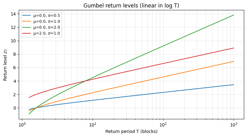
\mathbb{E}[X] = \mu + \gamma\sigma,\qquad \mathrm{Var}[X] = \frac{\pi^2}{6}\sigma^2,\qquad \text{skew} = \frac{12\sqrt{6}\,\zeta(3)}{\pi^3} \approx 1.1395.

(5)

Return level for return period $T$ (probability $1 - 1/T$ of not being exceeded in any one block):

z_T = \mu - \sigma \,\log\!\bigl(-\log(1 - 1/T)\bigr).

(6)

Note that $z_T$ grows linearly in $\log T$ — the signature linear-in-log return-level plot of the Gumbel.

Physical examples

Annual maxima of mid-latitude daily temperature, where the parent distribution is approximately Gaussian.
Annual peak river stages on regulated rivers (light upper tails after dam control).
Maximum daily wind speeds outside the tropics.
Maximum component lifetimes when the underlying failure-time law has an exponential tail.

When to reach for something else. Heavy-tailed phenomena like extreme precipitation, financial losses, earthquake magnitudes or catastrophic insurance claims are under-predicted by Gumbel — use Fréchet (ξ > 0). Hard physical caps (e.g. material strength, run-up height against a fixed seawall) are over-predicted — use Weibull (ξ < 0).

gumbel_grid = [
    dict(loc=0.0, scale=0.5),
    dict(loc=0.0, scale=1.0),
    dict(loc=0.0, scale=2.0),
    dict(loc=2.0, scale=1.0),
]
plot_pdf_cdf(
    GumbelType1GEVD,
    gumbel_grid,
    lambda p: f"μ={p['loc']:.1f}, σ={p['scale']:.1f}",
    "GumbelType1GEVD  (ξ = 0)",
    x_range=(-4.0, 10.0),
)
plot_return_levels(
    GumbelType1GEVD,
    gumbel_grid,
    lambda p: f"μ={p['loc']:.1f}, σ={p['scale']:.1f}",
    "Gumbel return levels (linear in log T)",
)

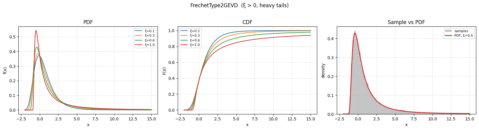
2. Fréchet (Type II, ξ > 0)¶

The Fréchet is the GEVD limit when the parent has a power-law (regularly varying) upper tail: $\mathbb{P}(X > x) \sim x^{-1/\xi}$ . The shape $\xi$ is the reciprocal of the tail index $\alpha$ :

\mathbb{P}(X > x) \sim x^{-\alpha},\qquad \alpha = 1/\xi.

(7)

Heavier tail $\Rightarrow$ larger $\xi$ $\Rightarrow$ smaller $\alpha$ .

Density and CDF. Using $z = (x-\mu)/\sigma$ and the support $x \ge \mu - \sigma/\xi$ ,

F(x) = \exp\!\left\{-\bigl(1 + \xi z\bigr)^{-1/\xi}\right\},\qquad f(x) = \tfrac{1}{\sigma}(1 + \xi z)^{-(1/\xi + 1)} F(x).

(8)

Moments are partial. The $k$ -th moment exists iff $\xi < 1/k$ :

\mathbb{E}[X] = \mu + \tfrac{\sigma}{\xi}\bigl(\Gamma(1-\xi) - 1\bigr),\quad \xi < 1.

(9)

For $\xi \ge 1$ the mean is infinite; for $\xi \ge 1/2$ the variance blows up. That divergence is not a numerical artefact — it is the defining behaviour of the family.

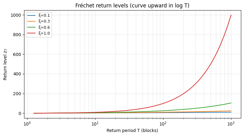
Return level.

z_T = \mu + \tfrac{\sigma}{\xi}\Bigl[\bigl(-\log(1-1/T)\bigr)^{-\xi} - 1\Bigr].

(10)

On a $\log T$ axis, $z_T$ curves upward — the hallmark of heavy tails.

Physical examples

Daily precipitation extremes (the textbook heavy-tail meteorological variable).
Earthquake magnitudes (Gutenberg–Richter is a power law).
Insurance claim sizes, especially catastrophic claims.
Internet packet interarrival sizes and file size distributions.
Tropical cyclone wind speeds and storm surges in the heavy-tail regime.

When to reach for something else. Bounded physical quantities (max wave run-up against a seawall of finite height, peak strain against the breaking limit of a beam) cannot have a power-law tail — use Weibull. Light-tailed temperature data fits Gumbel better; if you fit Fréchet there it will say $\xi \approx 0$ but use up a degree of freedom unnecessarily.

frechet_grid = [
    dict(loc=0.0, scale=1.0, concentration=0.1),
    dict(loc=0.0, scale=1.0, concentration=0.3),
    dict(loc=0.0, scale=1.0, concentration=0.6),
    dict(loc=0.0, scale=1.0, concentration=1.0),
]
plot_pdf_cdf(
    FrechetType2GEVD,
    frechet_grid,
    lambda p: f"ξ={p['concentration']:.1f}",
    "FrechetType2GEVD  (ξ > 0, heavy tails)",
    x_range=(-2.0, 15.0),
)
plot_return_levels(
    FrechetType2GEVD,
    frechet_grid,
    lambda p: f"ξ={p['concentration']:.1f}",
    "Fréchet return levels (curve upward in log T)",
)

3. Weibull (Type III, ξ < 0)¶

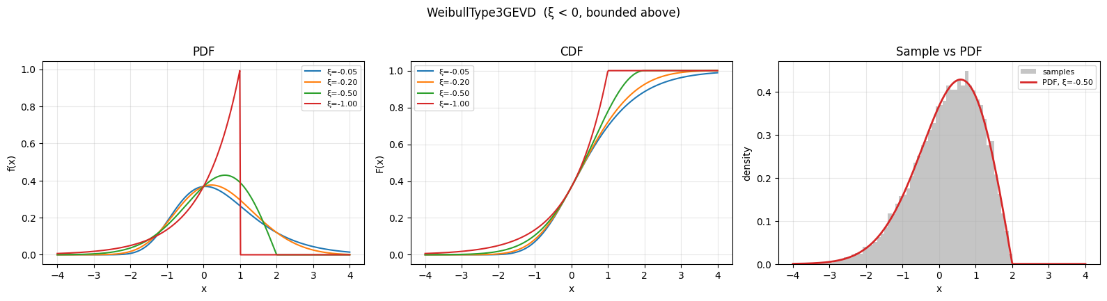
The reversed Weibull is the GEVD limit when the parent distribution has a finite right endpoint. Support is upper-bounded:

x \le x_{\sup} \;=\; \mu - \sigma/\xi \quad (\xi < 0).

(11)

As $\xi \to 0^-$ the upper endpoint recedes to $+\infty$ and we recover Gumbel.

Density and CDF are the same Coles formula as Fréchet, restricted to $\xi < 0$ . With $z = (x-\mu)/\sigma$ ,

F(x) = \exp\!\bigl\{-(1 + \xi z)^{-1/\xi}\bigr\},\qquad x \le \mu - \sigma/\xi.

(12)

All moments exist because the support is bounded:

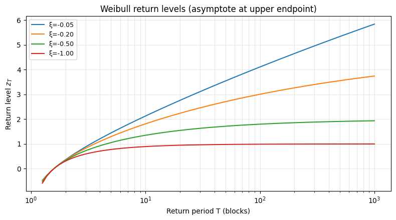
\mathbb{E}[X] = \mu + \tfrac{\sigma}{\xi}\bigl(\Gamma(1-\xi) - 1\bigr) \quad \text{(finite for all }\xi < 0\text{)}.

(13)

Return level. Same closed form as Fréchet,

z_T = \mu + \tfrac{\sigma}{\xi}\Bigl[\bigl(-\log(1-1/T)\bigr)^{-\xi} - 1\Bigr],

(14)

but on a $\log T$ axis it flattens and asymptotes to the upper endpoint $\mu - \sigma/\xi$ .

Physical examples

Maximum strength of brittle materials (there is a hard breaking stress).
Human lifespan (biological maximum near 120 years).
Maximum surge height against a fixed seawall: any excess simply spills over.
Maximum power output of a renewable source with a hard-rated capacity.
Reliability extremes when the failure mechanism has a deterministic upper bound.

When to reach for something else. If your “cap” is probabilistic rather than physical (rare crossings still happen) you may be in the Gumbel regime. If your data show no sign of saturating — return-level plot keeps climbing on a log axis — the data probably does not justify the bounded fit; let GEVD pick $\xi$ rather than forcing $\xi < 0$ .

weibull_grid = [
    dict(loc=0.0, scale=1.0, concentration=-0.05),
    dict(loc=0.0, scale=1.0, concentration=-0.2),
    dict(loc=0.0, scale=1.0, concentration=-0.5),
    dict(loc=0.0, scale=1.0, concentration=-1.0),
]
plot_pdf_cdf(
    WeibullType3GEVD,
    weibull_grid,
    lambda p: f"ξ={p['concentration']:.2f}",
    "WeibullType3GEVD  (ξ < 0, bounded above)",
    x_range=(-4.0, 4.0),
)
plot_return_levels(
    WeibullType3GEVD,
    weibull_grid,
    lambda p: f"ξ={p['concentration']:.2f}",
    "Weibull return levels (asymptote at upper endpoint)",
)

4. The unifying GEVD¶

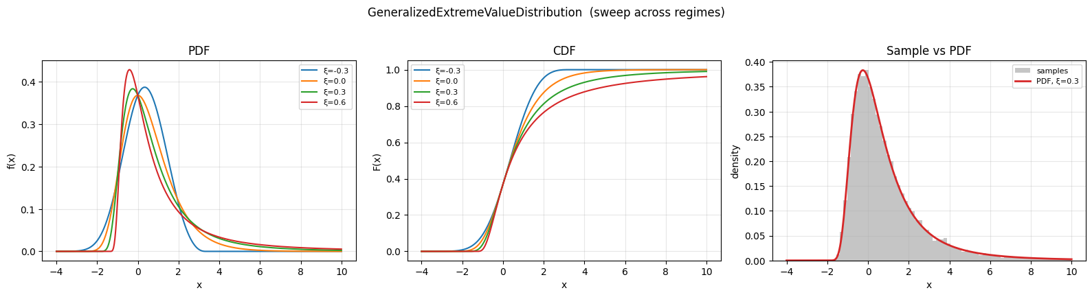
GeneralizedExtremeValueDistribution(loc, scale, concentration) exposes the full $(\mu,\sigma,\xi)$ family in one class. Use this when you do not know the tail regime a priori and want the data to choose $\xi$ . The implementation branches on $|\xi| < 10^{-7}$ and falls through to the Gumbel limit, so $\xi = 0$ is numerically safe.

In a Bayesian fit one typically places a weakly informative prior on $\xi$ (e.g. $\mathcal{N}(0, 0.3)$ ) so all three regimes are reachable, and reads off the posterior to decide which one the data prefers. Coles (2001, §3) is the standard reference for the diagnostics (return-level plot, PP/QQ plot, profile likelihood for $\xi$ ).

Why have all three sub-classes too? The GumbelType1GEVD, FrechetType2GEVD, WeibullType3GEVD classes hard-encode the tail regime via arg_constraints. They are:

useful for priors — if you have strong reason to believe $\xi > 0$ (precipitation), constraining the model removes mass from the wrong half-line and improves identifiability;
faster to sample and more numerically stable in their respective regimes;
cleaner in NumPyro models, since numpyro.sample("xi", Normal(0, 0.3)) can be replaced by a constrained scale-only fit.

The full GEVD is the right default when you are exploring; the typed sub-classes are the right default when you are committing to a regime.

gevd_grid = [
    dict(loc=0.0, scale=1.0, concentration=-0.3),
    dict(loc=0.0, scale=1.0, concentration=0.0),
    dict(loc=0.0, scale=1.0, concentration=0.3),
    dict(loc=0.0, scale=1.0, concentration=0.6),
]
plot_pdf_cdf(
    GeneralizedExtremeValueDistribution,
    gevd_grid,
    lambda p: f"ξ={p['concentration']:.1f}",
    "GeneralizedExtremeValueDistribution  (sweep across regimes)",
    x_range=(-4.0, 10.0),
)
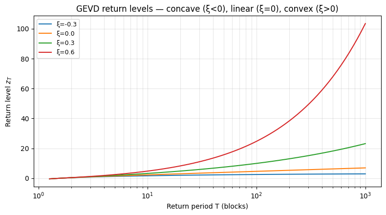
plot_return_levels(
    GeneralizedExtremeValueDistribution,
    gevd_grid,
    lambda p: f"ξ={p['concentration']:.1f}",
    "GEVD return levels — concave (ξ<0), linear (ξ=0), convex (ξ>0)",
)

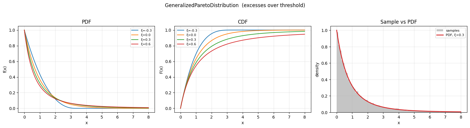
5. Generalized Pareto (POT)¶

The Pickands–Balkema–de Haan theorem says: if $X$ lies in the domain of attraction of a GEVD with shape $\xi$ , then for a high enough threshold $u$ the conditional excess

Y = X - u \mid X > u

(15)

is approximately distributed as a Generalized Pareto with the same $\xi$ and a scale $\sigma_u$ that depends on $u$ . Crucially, $\sigma_u$ varies with $u$ via the threshold-stability relation

\sigma_{u_2} = \sigma_{u_1} + \xi(u_2 - u_1),

(16)

which means a non-trivial slope of $\sigma_u$ vs $u$ on a mean-residual-life plot is a sign that the asymptotic POT regime has not yet kicked in — pick a higher threshold.

Density and CDF (with $y \ge 0$ , additionally $y \le -\sigma/\xi$ if $\xi<0$ ):

F(y) = \begin{cases} 1 - \bigl(1 + \xi y/\sigma\bigr)^{-1/\xi}, & \xi \neq 0,\\ 1 - e^{-y/\sigma}, & \xi = 0, \end{cases}\qquad f(y) = \tfrac{1}{\sigma}\bigl(1 + \xi y/\sigma\bigr)^{-(1/\xi + 1)}.

(17)

Mean and variance (when finite — same $\xi$ -thresholds as Fréchet):

\mathbb{E}[Y] = \frac{\sigma}{1-\xi},\quad \xi < 1,\qquad \mathrm{Var}[Y] = \frac{\sigma^2}{(1-\xi)^2(1-2\xi)},\quad \xi < 1/2.

(18)

Return level for the $T$ -block return level under POT, with rate $\zeta_u = \mathbb{P}(X > u)$ and number of blocks $n_y$ per year (or per any rate unit):

z_T = u + \frac{\sigma}{\xi}\Bigl[(T n_y \zeta_u)^{\xi} - 1\Bigr].

(19)

(A pure GPD has no per-block notion of return period on its own — it is always combined with the rate of threshold exceedances.)

Physical examples

Storm-surge heights above the 95th percentile: more data than annual maxima, same tail in the limit.
Significant wave heights above a nuisance threshold.
Financial losses above value-at-risk: GPD is the workhorse for expected shortfall.
Wildfire burn-area exceedances above a regulatory threshold.
Rainfall accumulations above a flood-relevant cutoff.

When to reach for something else. If you naturally have block maxima (one observation per block, e.g. annual peak), use GEVD directly — pretending each annual max is a “threshold exceedance” wastes a degree of freedom. If your threshold is too low the GPD fit is biased; if it is too high the variance blows up. The threshold-selection step (next two notebooks in this series) is where most of the modelling effort goes.

gpd_grid = [
    dict(scale=1.0, concentration=-0.3),
    dict(scale=1.0, concentration=0.0),
    dict(scale=1.0, concentration=0.3),
    dict(scale=1.0, concentration=0.6),
]
plot_pdf_cdf(
    GeneralizedParetoDistribution,
    gpd_grid,
    lambda p: f"ξ={p['concentration']:.1f}",
    "GeneralizedParetoDistribution  (excesses over threshold)",
    x_range=(0.0, 8.0),
)

6. Comparison: same μ, σ; varying ξ¶

Putting all three GEVD types on a single axes makes the role of $\xi$ visible at a glance. We hold $\mu = 0$ , $\sigma = 1$ and vary $\xi$ from -0.4 (Weibull, bounded above at $1/0.4 = 2.5$ ) to +0.4 (Fréchet, heavy upper tail).

fig, axes = plt.subplots(1, 2, figsize=(13, 4.5))
xs = jnp.linspace(-3.5, 8.0, 600)
xis = [-0.4, -0.2, 0.0, 0.2, 0.4]
colors = plt.colormaps["coolwarm"](np.linspace(0.05, 0.95, len(xis)))
for xi, color in zip(xis, colors, strict=True):
    d = GeneralizedExtremeValueDistribution(loc=0.0, scale=1.0, concentration=xi)
    axes[0].plot(xs, jnp.exp(d.log_prob(xs)), color=color, label=f"ξ={xi:+.1f}")
    axes[1].plot(xs, d.cdf(xs), color=color, label=f"ξ={xi:+.1f}")
for ax in axes:
    ax.grid(True, alpha=0.3)
    ax.set_xlabel("x")
    ax.legend(fontsize=9)
axes[0].set_ylabel("f(x)")
axes[0].set_title("PDF — same (μ, σ); varying ξ")
axes[1].set_ylabel("F(x)")
axes[1].set_title("CDF — same (μ, σ); varying ξ")
plt.tight_layout()
plt.show()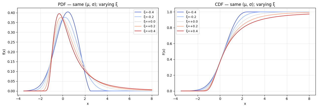

Read this figure as: negative ξ truncates the upper tail, positive ξ inflates it. The kink in the negative-ξ PDF is where the support hits $\mu - \sigma/\xi$ .

7. Comparison: GEVD vs GPD on a return-level axis¶

A side-by-side return-level plot makes the scaling differences concrete. We use a per-block exceedance rate of $\zeta_u = 0.05$ (one event in twenty blocks above the threshold) and compare the GEVD return level $z_T = \mu + \frac{\sigma}{\xi}\bigl[(-\log(1-1/T))^{-\xi} - 1\bigr]$ with the POT version $z_T = u + \frac{\sigma}{\xi}\bigl[(T \zeta_u)^{\xi} - 1\bigr]$ at threshold $u = 0$ .

The two curves should line up in their tails — that is the Pickands–Balkema–de Haan theorem in graphical form.

fig, ax = plt.subplots(figsize=(8, 5))
periods = jnp.logspace(0.1, 3, 80)
xis = [-0.2, 0.0, 0.2]
colors = ["tab:blue", "tab:gray", "tab:red"]
zeta_u = 0.05
u = 0.0
for xi, c in zip(xis, colors, strict=True):
    gev = GeneralizedExtremeValueDistribution(loc=0.0, scale=1.0, concentration=xi)
    gpd = GeneralizedParetoDistribution(scale=1.0, concentration=xi)
    rl_gev = gev.return_level(periods)
    safe_xi = jnp.where(jnp.abs(xi) < 1e-7, 1.0, xi)
    rl_pot = jnp.where(
        jnp.abs(xi) < 1e-7,
        u + 1.0 * jnp.log(periods * zeta_u),
        u + (1.0 / safe_xi) * (jnp.power(periods * zeta_u, safe_xi) - 1.0),
    )
    ax.plot(periods, rl_gev, color=c, ls="-", label=f"GEVD ξ={xi:+.1f}")
    ax.plot(periods, rl_pot, color=c, ls="--", label=f"POT ξ={xi:+.1f}")
ax.set_xscale("log")
ax.set_xlabel("Return period T (blocks)")
ax.set_ylabel("Return level $z_T$")
ax.grid(True, which="both", alpha=0.3)
ax.legend(fontsize=8, ncol=2)
ax.set_title("GEVD vs POT return levels — same ξ, different parameterisations")
plt.tight_layout()
plt.show()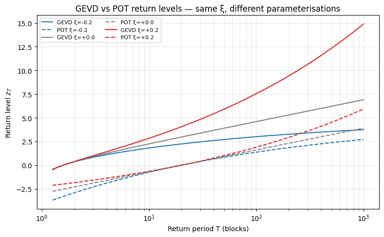

What’s next¶

The follow-up notebooks in this series demonstrate end-to-end workflows:

GEVD on annual maxima — synthetic daily series, xtremax.extraction.temporal_block_maxima, NumPyro NUTS, posterior return-level bands.
Fréchet on heavy-tailed precipitation — same flow as (1) with a Pareto-mixture parent and a comparison against a misspecified Gumbel fit.
Weibull on bounded extremes — same flow as (1) on a capped synthetic process, with the upper-endpoint posterior $\mu - \sigma/\xi$ as the headline quantity.
GPD via peaks-over-threshold — quantile_threshold + decluster_runs + a NumPyro GPD fit, with a mean-residual-life plot for threshold sensitivity.
Quantile-regression threshold + GPD — non-stationary thresholds via XarrayQuantileRegressor, residual GPD on the resulting exceedances.

Reading list

Coles, An Introduction to Statistical Modeling of Extreme Values, Springer, 2001 — the standard textbook; chapters 3 (GEVD), 4 (POT), 6 (Bayesian).
Embrechts, Klüppelberg & Mikosch, Modelling Extremal Events, Springer, 1997 — the financial/insurance perspective.
Beirlant, Goegebeur, Segers & Teugels, Statistics of Extremes, Wiley, 2004 — a more comprehensive theoretical reference.