GPD via Peaks-Over-Threshold

This notebook walks the canonical peaks-over-threshold (POT) pipeline. Instead of one observation per year (the block-maxima approach of the previous three notebooks), POT keeps every exceedance over a high threshold $u$ and models the conditional excesses with a Generalized Pareto Distribution.

POT is the workhorse parameterisation in finance, hydrology and reliability whenever you have more data than you would get from annual maxima alone — which is essentially always.

What we cover

Theory. The Pickands–Balkema–de Haan theorem; the GPD log-likelihood; threshold-stability and the mean-residual-life plot.
Threshold selection. quantile_threshold at the 95th percentile, plus a sensitivity sweep to show how the posterior on $\xi$ depends on $u$ .
Declustering. Why naïve POT fails on temporally correlated data, and how decluster_runs enforces independence.
Bayesian fit. NumPyro NUTS over $(\sigma, \xi)$ with weakly informative priors.
Return levels. The Poisson-GPD compound that gives the per-year return level.

import subprocess
import sys


try:
    import google.colab  # noqa: F401

    IN_COLAB = True
except ImportError:
    IN_COLAB = False

if IN_COLAB:
    subprocess.run(
        [
            sys.executable,
            "-m",
            "pip",
            "install",
            "-q",
            "xtremax @ git+https://github.com/jejjohnson/xtremax@main",
        ],
        check=True,
    )

import os


# Force two host devices so the two MCMC chains run in parallel. This sets an
# XLA flag that must be configured *before* JAX initialises, so it has to run
# before any `import jax` (importing numpyro also imports jax). Setting
# XLA_FLAGS directly is equivalent to numpyro.set_host_device_count(2) but is
# robust to import order.
os.environ.setdefault("XLA_FLAGS", "--xla_force_host_platform_device_count=2")

import warnings


warnings.filterwarnings("ignore", message=r".*IProgress.*")

import jax
import jax.numpy as jnp
import matplotlib.pyplot as plt
import numpy as np
import numpyro
import numpyro.distributions as ndist
import pandas as pd
import xarray as xr
from numpyro.infer import MCMC, NUTS
from numpyro.infer.initialization import init_to_median

from xtremax.distributions import GeneralizedParetoDistribution
from xtremax.extraction import decluster_runs, quantile_threshold


KEY = jax.random.PRNGKey(0)

import importlib.util


try:
    from IPython import get_ipython

    ipython = get_ipython()
except ImportError:
    ipython = None

if ipython is not None and importlib.util.find_spec("watermark") is not None:
    ipython.run_line_magic("load_ext", "watermark")
    ipython.run_line_magic(
        "watermark",
        "-v -m -p jax,numpy,matplotlib,numpyro,xarray,xtremax",
    )
else:
    print("watermark extension not installed; skipping reproducibility readout.")

Python implementation: CPython
Python version       : 3.12.3
IPython version      : 9.10.0

jax       : 0.10.1
numpy     : 2.4.4
matplotlib: 3.10.8
numpyro   : 0.21.0
xarray    : 2026.4.0
xtremax   : 0.0.0

Compiler    : GCC 13.3.0
OS          : Linux
Release     : 6.18.5
Machine     : x86_64
Processor   : x86_64
CPU cores   : 4
Architecture: 64bit

1. Pickands–Balkema–de Haan and the GPD¶

Suppose $X_1, X_2, \ldots$ are i.i.d. from a parent CDF $F$ in the GEVD domain of attraction with shape $\xi$ . Define the conditional excess distribution at threshold $u$ :

F_u(y) \;:=\; \mathbb{P}(X - u \le y \mid X > u) \;=\; \frac{F(u + y) - F(u)}{1 - F(u)},\qquad y \ge 0.

(1)

The Pickands–Balkema–de Haan (1974/1975) theorem says: there exists a positive function $\sigma_u$ such that, as $u$ approaches the right endpoint $x_F$ ,

\sup_{0 \le y < x_F - u} \bigl| F_u(y) - H(y;\,\sigma_u, \xi) \bigr| \;\xrightarrow[u \to x_F]{} \;0,

(2)

where $H$ is the Generalized Pareto CDF

H(y;\,\sigma, \xi) \;=\; \begin{cases} 1 - \bigl(1 + \xi y/\sigma\bigr)^{-1/\xi}, & \xi \neq 0, \\[4pt] 1 - e^{-y/\sigma}, & \xi = 0, \end{cases}

(3)

defined on $y \ge 0$ (and additionally $y \le -\sigma/\xi$ if $\xi < 0$ ).

Three crucial implications.

The shape parameter is shared. The $\xi$ in the GPD is the same $\xi$ that appears in the GEVD limit of $F$ . Block-maxima fits and POT fits should agree on $\xi$ (and they often do — that is a nice sanity check).
Threshold stability. If $X - u_1$ is GPD with parameters $(\sigma_{u_1}, \xi)$ and $u_2 > u_1$ , then $X - u_2$ is also GPD with the same $\xi$ and shifted scale
$\sigma_{u_2} \;=\; \sigma_{u_1} + \xi(u_2 - u_1).$
(4)
A non-trivial slope of $\sigma_u$ vs $u$ in fitted parameters is a sign that the asymptotic POT regime has not kicked in — raise the threshold.
The mean excess is linear. Define $e(u) := \mathbb{E}[X - u \mid X > u]$ . For a GPD with $\xi < 1$ ,
$e(u) \;=\; \frac{\sigma + \xi u}{1 - \xi},$
(5)
a linear function of the threshold. The empirical mean-excess plot should therefore be linear above the asymptotic threshold — a famous diagnostic.

Log-likelihood. Given exceedances $y_1, \ldots, y_k$ ,

\ell(\sigma, \xi) \;=\; -k\,\log\sigma \;-\; \bigl(1/\xi + 1\bigr)\sum_{i=1}^{k} \log\!\bigl(1 + \xi y_i/\sigma\bigr).

(6)

This is what GeneralizedParetoDistribution.log_prob evaluates inside NumPyro.

2. Synthetic temporally correlated daily series¶

We build a daily-stage process with: a smooth seasonal cycle, AR(1) persistence (so adjacent days are correlated — not i.i.d.), and Gaussian noise. POT pretends the exceedances are independent; we will see how this assumption fails on the raw series and how decluster_runs fixes it.

N_YEARS = 80
DAYS_PER_YEAR = 365
RNG = np.random.default_rng(20260429)

dates = pd.date_range("1945-01-01", periods=N_YEARS * DAYS_PER_YEAR, freq="D")
n = N_YEARS * DAYS_PER_YEAR
day_of_year = (dates.dayofyear - 1).to_numpy()
seasonal = 5.0 * np.sin(2 * np.pi * day_of_year / DAYS_PER_YEAR)

# AR(1) noise with persistence rho=0.6 — neighbouring days are correlated.
rho = 0.6
innovation = RNG.normal(0.0, 1.0, size=n)
ar1 = np.empty(n)
ar1[0] = innovation[0]
for t in range(1, n):
    ar1[t] = rho * ar1[t - 1] + innovation[t]
ar1 *= np.sqrt(1.0 - rho**2) * 4.0  # rescale to ~unit-variance times σ
daily = 10.0 + seasonal + ar1

series = xr.DataArray(daily, dims="time", coords={"time": dates})

fig, ax = plt.subplots(figsize=(11, 3.0))
ax.plot(series.time, series.values, lw=0.4, alpha=0.7, color="tab:blue")
ax.set_title("Synthetic AR(1) daily series with seasonal cycle (80 yr)")
ax.set_xlabel("date")
ax.set_ylabel("daily value")
ax.grid(True, alpha=0.3)
plt.tight_layout()
plt.show()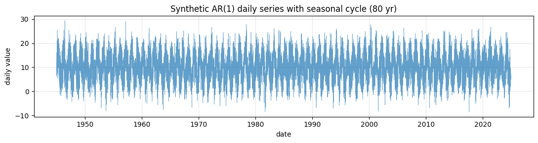

3. Threshold selection at the 95th percentile¶

u = float(quantile_threshold(series, 0.95))
print(f"95th percentile threshold u = {u:.3f}")

raw_exceedances = (series.where(series > u) - u).dropna("time")
print(f"Raw (non-declustered) exceedances: {raw_exceedances.sizes['time']}")

fig, ax = plt.subplots(figsize=(11, 3.0))
ax.plot(series.time, series.values, lw=0.3, alpha=0.4, color="tab:blue", label="daily")
ax.axhline(u, color="tab:red", lw=1.5, ls="--", label=f"u = {u:.2f}")
ax.scatter(
    raw_exceedances.time,
    raw_exceedances.values + u,
    color="tab:red",
    s=8,
    zorder=3,
    label="exceedance days",
)
ax.set_xlim(series.time.values[0], series.time.values[365 * 5])
ax.set_xlabel("date")
ax.set_ylabel("daily value")
ax.set_title("First 5 years — raw exceedances cluster temporally")
ax.legend(fontsize=8)
ax.grid(True, alpha=0.3)
plt.tight_layout()
plt.show()

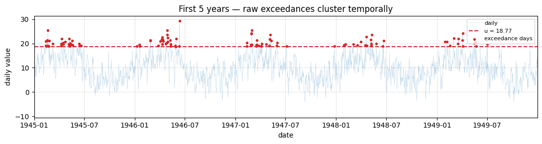
95th percentile threshold u = 18.774
Raw (non-declustered) exceedances: 1460

Why declustering matters¶

The plot above shows the issue. Adjacent exceedance days come from the same extreme weather event, and they are highly correlated — fitting a GPD to all of them violates the i.i.d. assumption and produces a spuriously narrow posterior. The classical fix is the runs method: collapse each contiguous run of exceedances into a single “event” (typically the maximum within the run), keeping only one observation per cluster.

declustered = decluster_runs(series, threshold=u, reduction="max")
declustered_excess = declustered.dropna("time") - u
print(f"Declustered exceedances: {declustered_excess.sizes['time']}")
print(
    f"Cluster reduction:       "
    f"{raw_exceedances.sizes['time']} → {declustered_excess.sizes['time']} "
    f"({100 * declustered_excess.sizes['time'] / raw_exceedances.sizes['time']:.1f}%)"
)

excess = jnp.asarray(declustered_excess.values)

Declustered exceedances: 847
Cluster reduction:       1460 → 847 (58.0%)

4. Mean-residual-life (mean-excess) plot¶

The mean-excess function $e(u) = \mathbb{E}[X - u \mid X > u]$ should be linear in $u$ above the asymptotic threshold. We plot the empirical $\hat e(u)$ over a sweep of candidate thresholds; we want to identify a value above which the curve is roughly linear.

threshold_grid = np.linspace(np.quantile(daily, 0.80), np.quantile(daily, 0.999), 60)
mean_excess = []
n_above = []
ci_half_width = []
for u_test in threshold_grid:
    above = daily[daily > u_test] - u_test
    if len(above) > 5:
        mean_excess.append(above.mean())
        n_above.append(len(above))
        ci_half_width.append(1.96 * above.std(ddof=1) / np.sqrt(len(above)))
    else:
        mean_excess.append(np.nan)
        n_above.append(0)
        ci_half_width.append(np.nan)
mean_excess = np.asarray(mean_excess)
ci_half_width = np.asarray(ci_half_width)

fig, ax = plt.subplots(figsize=(8, 4.5))
ax.plot(threshold_grid, mean_excess, color="tab:blue")
ax.fill_between(
    threshold_grid,
    mean_excess - ci_half_width,
    mean_excess + ci_half_width,
    alpha=0.2,
    color="tab:blue",
    label="95% CI",
)
ax.axvline(u, color="tab:red", lw=2, ls="--", label=f"chosen u = {u:.2f}")
ax.set_xlabel("threshold u")
ax.set_ylabel(r"empirical mean excess $\hat e(u)$")
ax.set_title("Mean-residual-life plot")
ax.grid(True, alpha=0.3)
ax.legend()
plt.tight_layout()
plt.show()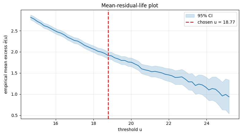

Reading this:

Linear region above some threshold: the asymptotic GPD regime has kicked in. The slope is $\xi/(1-\xi)$ and the intercept is $\sigma_0/(1-\xi)$ .
Curved or noisy region below: the threshold is too low (non-tail observations contaminate) or above (variance is too high — fewer data).
The plotted 95% confidence band widens to the right because the right-tail samples thin out; this is the small-sample end.

The chosen $u$ should sit comfortably inside the linear region and have enough exceedances above it for a stable fit — there is genuine art here, and the plot is a sanity check, not a recipe.

5. Bayesian GPD fit¶

Model. With independent declustered excesses $y_i = z_i - u$ ,

y_i \mid \sigma, \xi \;\sim\; \mathrm{GPD}(\sigma, \xi).

(7)

Priors.

$\sigma \sim \mathrm{HalfNormal}(2 \bar y)$ , where $\bar y$ is the empirical mean excess. Half-normal is positive; the scale is comfortably wider than any plausible value.
$\xi \sim \mathcal{N}(0, 0.25)$ , a weakly informative prior covering the physically reasonable range $[-0.5, +0.5]$ .

sigma_loc = float(jnp.mean(excess))


def gpd_model(excess, sigma_prior_scale):
    sigma = numpyro.sample("sigma", ndist.HalfNormal(sigma_prior_scale * 2))
    xi = numpyro.sample("xi", ndist.Normal(0.0, 0.25))
    numpyro.sample(
        "obs",
        GeneralizedParetoDistribution(scale=sigma, concentration=xi),
        obs=excess,
    )


# target_accept_prob is pushed to 0.99 (smaller leapfrog steps) with a longer
# warmup so NUTS resolves the funnel-like (sigma, xi) geometry without
# divergent transitions. init_to_median starts both chains in the bulk.
kernel = NUTS(gpd_model, target_accept_prob=0.99, init_strategy=init_to_median)
mcmc = MCMC(kernel, num_warmup=3000, num_samples=2000, num_chains=2, progress_bar=False)
mcmc.run(KEY, excess=excess, sigma_prior_scale=sigma_loc, extra_fields=("diverging",))
mcmc.print_summary(prob=0.95)

# Fail fast on divergences: divergent transitions mean HMC is not exploring the
# posterior geometry, so the samples (and any return levels built from them)
# would be biased. Surface the count and refuse to proceed if it is nonzero.
n_divergences = int(mcmc.get_extra_fields()["diverging"].sum())
print(f"\nNumber of divergences: {n_divergences}")
if n_divergences > 0:
    raise RuntimeError(
        f"NUTS reported {n_divergences} divergent transition(s); retune the "
        "sampler (raise target_accept_prob, add warmup, reparameterise) before "
        "consuming the posterior."
    )

posterior = mcmc.get_samples()


                mean       std    median      2.5%     97.5%     n_eff     r_hat
     sigma      2.54      0.10      2.54      2.34      2.75   1095.19      1.00
        xi     -0.18      0.02     -0.19     -0.23     -0.14   1113.05      1.00

Number of divergences: 0

Number of divergences: 0

fig, axes = plt.subplots(1, 2, figsize=(11, 3.6))
for ax, name, samples in zip(
    axes,
    ["sigma", "xi"],
    [posterior["sigma"], posterior["xi"]],
    strict=True,
):
    ax.hist(np.asarray(samples), bins=40, density=True, color="tab:blue", alpha=0.6)
    ax.axvline(
        float(jnp.median(samples)),
        color="tab:red",
        lw=2,
        label=f"median = {float(jnp.median(samples)):.3f}",
    )
    ax.set_title(rf"GPD posterior $\{name}$")
    ax.grid(True, alpha=0.3)
    ax.legend(fontsize=8)
plt.tight_layout()
plt.show()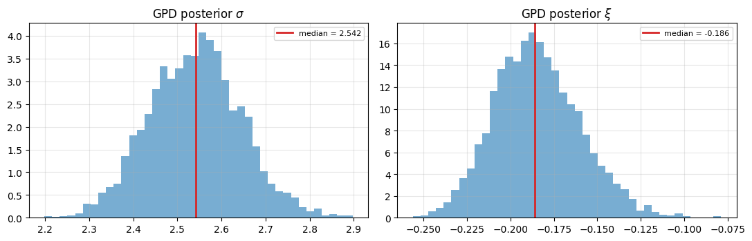

6. Threshold-sensitivity sweep¶

How robust is the inference to the choice of $u$ ? We re-fit the GPD at a sweep of candidate thresholds and plot the posterior median (with 95% CI) of $\xi$ as a function of $u$ . Threshold stability says $\xi$ should be approximately constant above the asymptotic threshold; a flat plateau is evidence that the chosen $u$ is in the right regime.

def fit_at_threshold(u_test, key):
    excess_t = (
        declustered_runs := decluster_runs(series, threshold=u_test, reduction="max")
    )
    excess_t = declustered_runs.dropna("time") - u_test
    if excess_t.sizes["time"] < 30:
        return None
    excess_t = jnp.asarray(excess_t.values)
    s_loc = float(jnp.mean(excess_t))
    kernel_t = NUTS(gpd_model, target_accept_prob=0.95, init_strategy=init_to_median)
    mcmc_t = MCMC(
        kernel_t, num_warmup=600, num_samples=800, num_chains=2, progress_bar=False
    )
    mcmc_t.run(key, excess=excess_t, sigma_prior_scale=s_loc)
    return mcmc_t.get_samples()


sweep_quantiles = [0.85, 0.88, 0.90, 0.93, 0.95, 0.97, 0.99]
sweep_us = [float(quantile_threshold(series, q)) for q in sweep_quantiles]
sweep_keys = jax.random.split(KEY, len(sweep_us))
sweep_xi_med = []
sweep_xi_lo = []
sweep_xi_hi = []
sweep_n = []
for u_test, k in zip(sweep_us, sweep_keys, strict=True):
    decl = decluster_runs(series, threshold=u_test, reduction="max")
    excess_t_da = decl.dropna("time") - u_test
    excess_t = jnp.asarray(excess_t_da.values)
    sweep_n.append(int(excess_t_da.sizes["time"]))
    s_loc = float(jnp.mean(excess_t))
    kernel_t = NUTS(gpd_model, target_accept_prob=0.95, init_strategy=init_to_median)
    mcmc_t = MCMC(
        kernel_t, num_warmup=600, num_samples=800, num_chains=2, progress_bar=False
    )
    mcmc_t.run(k, excess=excess_t, sigma_prior_scale=s_loc)
    s = mcmc_t.get_samples()["xi"]
    sweep_xi_med.append(float(jnp.median(s)))
    sweep_xi_lo.append(float(jnp.quantile(s, 0.025)))
    sweep_xi_hi.append(float(jnp.quantile(s, 0.975)))

sweep_xi_med = np.asarray(sweep_xi_med)
sweep_xi_lo = np.asarray(sweep_xi_lo)
sweep_xi_hi = np.asarray(sweep_xi_hi)

fig, ax = plt.subplots(figsize=(9, 4.5))
ax.fill_between(
    sweep_us,
    sweep_xi_lo,
    sweep_xi_hi,
    alpha=0.25,
    color="tab:blue",
    label="95% credible band",
)
ax.plot(
    sweep_us,
    sweep_xi_med,
    color="tab:blue",
    marker="o",
    lw=2,
    label=r"posterior median $\xi$",
)
ax.axhline(0, color="tab:gray", lw=1, ls="--")
ax.axvline(u, color="tab:red", lw=1.5, ls=":", label=f"chosen u = {u:.2f}")
for u_test, q, ndecl in zip(sweep_us, sweep_quantiles, sweep_n, strict=True):
    ax.annotate(
        f"q={q:.2f}\nn={ndecl}",
        xy=(u_test, ax.get_ylim()[1]),
        xytext=(0, -10),
        textcoords="offset points",
        ha="center",
        fontsize=7,
        color="tab:gray",
    )
ax.set_xlabel("threshold u")
ax.set_ylabel(r"GPD shape posterior $\xi(u)$")
ax.set_title("Threshold sensitivity of the GPD shape")
ax.grid(True, alpha=0.3)
ax.legend(fontsize=8, loc="lower right")
plt.tight_layout()
plt.show()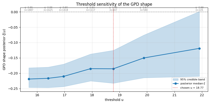

A flat curve says the asymptotic regime has kicked in and the chosen threshold sits in a stable region. A trending curve says you should pick a higher threshold (until the trend disappears or until the credible band blows up from too-few-exceedances). For our AR(1) Gaussian-tail process we expect $\xi \approx 0$ across the upper plateau.

7. Return levels via Poisson–GPD compound¶

A pure GPD models excess sizes, not the frequency of exceedances. To get the per-year return level you need the rate $\lambda_u$ of exceedances per year and combine the two as

z_T \;=\; u + \frac{\sigma}{\xi}\Bigl[(T \lambda_u)^{\xi} - 1\Bigr], \qquad \xi \neq 0,

(8)

i.e. “the level exceeded with probability $1/(T \lambda_u)$ given a threshold exceedance.” We use the empirical declustered rate

\hat\lambda_u \;=\; \text{(declustered exceedances)} / \text{(years of data)}.

(9)

years_of_data = (series.time.values[-1] - series.time.values[0]) / np.timedelta64(
    365, "D"
)
lambda_u = declustered_excess.sizes["time"] / years_of_data
print(f"Declustered events per year: λ_u = {lambda_u:.2f}")

periods = jnp.logspace(0.1, 3, 80)


def rl_pot(sigma, xi, T, u_val, lam):
    Tlam = T * lam
    safe_xi = jnp.where(jnp.abs(xi) < 1e-7, 1.0, xi)
    return jnp.where(
        jnp.abs(xi) < 1e-7,
        u_val + sigma * jnp.log(Tlam),
        u_val + (sigma / safe_xi) * (jnp.power(Tlam, safe_xi) - 1.0),
    )


rl_samples = jax.vmap(lambda s, x: rl_pot(s, x, periods, u, lambda_u))(
    posterior["sigma"], posterior["xi"]
)

# Empirical (Weissman) plotting positions for declustered exceedances
sorted_excess = np.sort(np.asarray(excess))
m = len(sorted_excess)
emp_periods = 1.0 / (lambda_u * (1 - np.arange(1, m + 1) / (m + 1)))

med = jnp.median(rl_samples, axis=0)
lo = jnp.quantile(rl_samples, 0.025, axis=0)
hi = jnp.quantile(rl_samples, 0.975, axis=0)

fig, ax = plt.subplots(figsize=(8, 5))
ax.fill_between(
    periods, lo, hi, alpha=0.25, color="tab:blue", label="95% credible band"
)
ax.plot(periods, med, color="tab:blue", lw=2, label="posterior median")
ax.scatter(
    emp_periods,
    sorted_excess + u,
    color="tab:red",
    zorder=3,
    label="empirical (declustered)",
)
ax.set_xscale("log")
ax.set_xlabel("Return period T (years)")
ax.set_ylabel("Return level $z_T$")
ax.set_title("Poisson-GPD return-level plot")
ax.grid(True, which="both", alpha=0.3)
ax.legend()
plt.tight_layout()
plt.show()

idx_100 = int(jnp.argmin(jnp.abs(periods - 100.0)))
print(f"100-year return level (posterior median): {float(med[idx_100]):.2f}")
print(
    f"95% credible interval:                    "
    f"[{float(lo[idx_100]):.2f}, {float(hi[idx_100]):.2f}]"
)

Declustered events per year: λ_u = 10.59

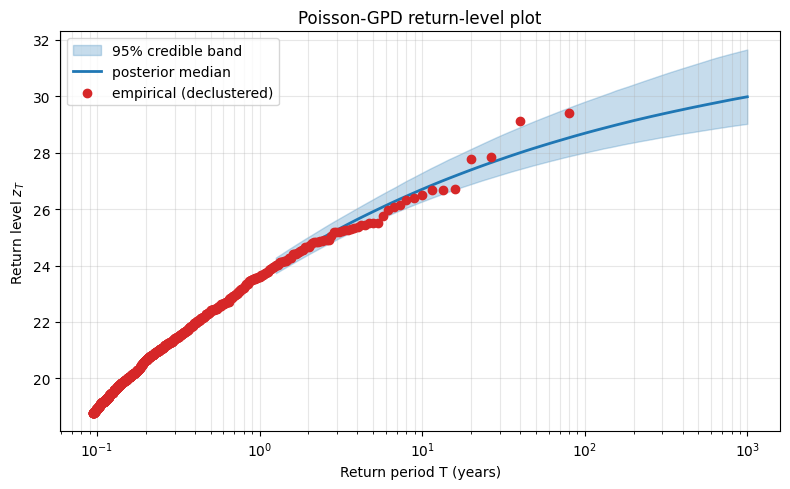
100-year return level (posterior median): 28.70
95% credible interval:                    [28.01, 29.82]

8. PP plot for the GPD fit¶

Same diagnostic as for the GEVD: order the excesses $y_{(1)} \le \ldots \le y_{(k)}$ , plot $\hat F(y_{(i)})$ vs $i/(k+1)$ .

sigma_med = float(jnp.median(posterior["sigma"]))
xi_med = float(jnp.median(posterior["xi"]))
fitted_gpd = GeneralizedParetoDistribution(scale=sigma_med, concentration=xi_med)
sorted_excess_jx = jnp.asarray(sorted_excess)
emp_p = (np.arange(1, m + 1)) / (m + 1)

fig, axes = plt.subplots(1, 2, figsize=(11, 4.5))
axes[0].plot([0, 1], [0, 1], color="tab:gray", lw=1)
axes[0].scatter(
    emp_p, np.asarray(fitted_gpd.cdf(sorted_excess_jx)), color="tab:blue", s=10
)
axes[0].set_xlabel("empirical $i/(k+1)$")
axes[0].set_ylabel(r"fitted $\hat H(y_{(i)})$")
axes[0].set_title("PP plot")
axes[0].grid(True, alpha=0.3)


# numpyro's GPD doesn't expose icdf, so build it from the closed form.
def gpd_quantile(p, sigma, xi):
    if abs(xi) < 1e-7:
        return -sigma * np.log(1 - p)
    return (sigma / xi) * ((1 - p) ** (-xi) - 1.0)


q_fit = np.asarray([gpd_quantile(p, sigma_med, xi_med) for p in emp_p])
mn, mx = sorted_excess.min(), sorted_excess.max()
axes[1].plot([mn, mx], [mn, mx], color="tab:gray", lw=1)
axes[1].scatter(q_fit, sorted_excess, color="tab:blue", s=10)
axes[1].set_xlabel(r"fitted quantile $\hat H^{-1}(p_i)$")
axes[1].set_ylabel(r"empirical $y_{(i)}$")
axes[1].set_title("QQ plot")
axes[1].grid(True, alpha=0.3)
plt.tight_layout()
plt.show()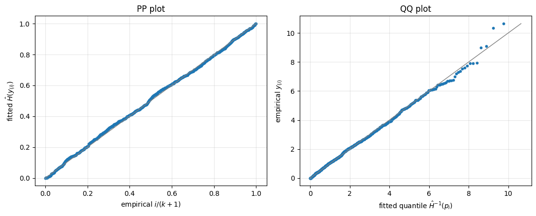

Takeaways¶

POT uses every exceedance, not just one per year. With AR(1) data and a 95th-percentile threshold we get hundreds of declustered events; the GPD posterior is correspondingly tight.
Decluster before fitting. Naïve POT on raw exceedances violates i.i.d. and produces a falsely narrow posterior. decluster_runs collapses each contiguous run into one event.
Validate the threshold. The mean-residual-life plot and the threshold-sensitivity sweep both target the same question — is $u$ high enough that the asymptotic regime has kicked in? — and give complementary visual answers.
Return levels need a rate. GPD on its own has no per-year scale; the Poisson-GPD compound multiplies the exceedance rate $\lambda_u$ into the return-period formula.

The next notebook generalises threshold selection to non-stationary data via XarrayQuantileRegressor, fitting a covariate-dependent threshold and feeding the residual exceedances into the same GPD.