Non-Stationary GEVD: Parametric Trend in μ(t)

The previous EVT notebooks all assumed stationarity — that the parameters $(\mu, \sigma, \xi)$ are constant across the record. In a warming climate, an aging asset, or a covariate-driven setting, this is wrong, and the resulting fit absorbs the non-stationarity into the wrong parameter (typically $\sigma$ ).

This notebook fits the simplest non-stationary GEVD: a parametric linear trend in the location parameter,

\mu(t) \;=\; \beta_0 + \beta_1\, t,

(1)

with $\sigma$ and $\xi$ held stationary. We generate annual block maxima from such a model on simulated daily data, fit the non-stationary version, and compare against a misspecified stationary fit.

What we cover

Theory. The non-stationary GEVD likelihood; why $\mu$ is the natural parameter to put a trend on; non-stationary return levels.
Synthetic 1D data. 80 years of daily values with a planted upward trend in the location.
Bayesian fit. NumPyro NUTS over $(\beta_0, \beta_1, \sigma, \xi)$ .
Stationary vs non-stationary. Side-by-side posteriors and return-level curves.
Recovery. Show that $\hat\beta_1$ matches the planted slope and that the non-stationary 100-yr return level rises with time at the right rate.

import subprocess
import sys


try:
    import google.colab  # noqa: F401

    IN_COLAB = True
except ImportError:
    IN_COLAB = False

if IN_COLAB:
    subprocess.run(
        [
            sys.executable,
            "-m",
            "pip",
            "install",
            "-q",
            "xtremax @ git+https://github.com/jejjohnson/xtremax@main",
        ],
        check=True,
    )

import warnings


warnings.filterwarnings("ignore", message=r".*IProgress.*")

import jax
import jax.numpy as jnp
import matplotlib.pyplot as plt
import numpy as np
import numpyro
import numpyro.distributions as ndist
import pandas as pd
import xarray as xr
from numpyro.infer import MCMC, NUTS
from numpyro.infer.initialization import init_to_median

from xtremax.distributions import GeneralizedExtremeValueDistribution


KEY = jax.random.PRNGKey(0)

import importlib.util


try:
    from IPython import get_ipython

    ipython = get_ipython()
except ImportError:
    ipython = None

if ipython is not None and importlib.util.find_spec("watermark") is not None:
    ipython.run_line_magic("load_ext", "watermark")
    ipython.run_line_magic(
        "watermark",
        "-v -m -p jax,numpy,matplotlib,numpyro,xarray,xtremax",
    )
else:
    print("watermark extension not installed; skipping reproducibility readout.")

Python implementation: CPython
Python version       : 3.12.3
IPython version      : 9.10.0

jax       : 0.10.1
numpy     : 2.4.4
matplotlib: 3.10.8
numpyro   : 0.21.0
xarray    : 2026.4.0
xtremax   : 0.0.0

Compiler    : GCC 13.3.0
OS          : Linux
Release     : 6.18.5
Machine     : x86_64
Processor   : x86_64
CPU cores   : 4
Architecture: 64bit

1. The non-stationary GEVD likelihood¶

In the stationary fit, every block maximum $z_i$ is i.i.d. from the same $\mathrm{GEVD}(\mu, \sigma, \xi)$ . The non-stationary version simply lets one or more parameters depend on a covariate $x_i$ (here, time):

z_i \mid x_i \;\sim\; \mathrm{GEVD}\!\bigl(\mu(x_i), \sigma(x_i), \xi(x_i)\bigr).

(2)

The log-likelihood is the obvious sum:

\ell\bigl(\boldsymbol\beta_\mu, \boldsymbol\beta_\sigma, \boldsymbol\beta_\xi\bigr) \;=\; \sum_{i=1}^{n} \log f_{\mathrm{GEVD}}\!\bigl(z_i;\, \mu(x_i), \sigma(x_i), \xi(x_i)\bigr).

(3)

Which parameters should you put a trend on? Coles (2001, §6) argues:

$\mu$ is the natural one. It is interpretable (the “central level” of the maxima) and trends in physical processes — warming, aging, sensor drift — typically shift the location of the tail.
$\sigma$ can be made covariate-dependent if there is a clear reason (e.g. the variance of a process scales with its mean). Use $\log\sigma(x) = \alpha_0 + \alpha_1 x$ to enforce positivity.
$\xi$ is dangerous to make non-stationary: it is already poorly identified in the stationary fit, and adding a regression on it usually leads to wide, unstable posteriors. Hold $\xi$ fixed unless you have a lot of data and a strong physical reason.

This notebook plants the trend in $\mu$ only — the cleanest case.

Return level under non-stationarity. Define the $T$ -block return level given the covariate as

z_T(x) \;=\; F^{-1}_{\mathrm{GEVD}}(1 - 1/T;\,\mu(x), \sigma, \xi) \;=\; \mu(x) + \frac{\sigma}{\xi}\Bigl[\bigl(-\log(1-1/T)\bigr)^{-\xi} - 1\Bigr].

(4)

Under a linear trend $\mu(x) = \beta_0 + \beta_1 x$ , the curve $z_T(x)$ is also linear in $x$ with the same slope $\beta_1$ — the trend translates the entire tail upward by an amount that does not depend on $T$ . (If $\sigma$ or $\xi$ also vary with $x$ , the slope changes with $T$ .)

2. Synthetic 80-year annual maxima¶

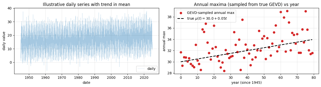
We want annual block maxima that follow $\mathrm{GEVD}(\mu(t), \sigma, \xi)$ with $\mu(t) = \beta_0 + \beta_1 t$ linear in years and $(\sigma, \xi) = (2.0, -0.10)$ stationary. The trend is $\beta_1 = 0.05$ per year — a noticeable warming over 80 years.

To make the planted truth exact, we sample the annual maxima directly from the declared non-stationary GEVD: for each year $t$ we draw

z_t \;\sim\; \mathrm{GEVD}\!\bigl(\mu(t) = \beta_0 + \beta_1 t,\; \sigma,\; \xi\bigr).

(5)

This matches the model’s $\mu(t) = \beta_0 + \beta_1 t$ structure exactly, so the “true” $(\sigma, \xi)$ overlays and the $z_T(t)$ return-level curve are genuine ground truth — not the approximate Fisher-Tippett-Gnedenko limit of a block-maxima procedure. We also synthesise a daily series with the same upward trend in its mean, purely to visualise the kind of process such maxima arise from, but the values used for fitting are the GEVD draws.

N_YEARS = 80
DAYS_PER_YEAR = 365
RNG = np.random.default_rng(20260429)

BETA0_TRUE = 30.0
BETA1_TRUE = 0.05
SIGMA_TRUE = 2.0
XI_TRUE = -0.10

# Year covariate: one block maximum per year, t = 0, 1, ..., N_YEARS - 1.
years = jnp.arange(N_YEARS, dtype=jnp.float32)

# Plant the truth EXACTLY: draw each annual maximum directly from the
# non-stationary GEVD with mu(t) = beta0 + beta1 * t and stationary (sigma, xi).
mu_true = BETA0_TRUE + BETA1_TRUE * years
key_data = jax.random.PRNGKey(23)
maxima = GeneralizedExtremeValueDistribution(
    loc=mu_true, scale=SIGMA_TRUE, concentration=XI_TRUE
).sample(key_data)

# A daily series with the same upward trend in its mean, for visualisation only.
dates = pd.date_range("1945-01-01", periods=N_YEARS * DAYS_PER_YEAR, freq="D")
n = N_YEARS * DAYS_PER_YEAR
day_of_year = (dates.dayofyear - 1).to_numpy()
year_index = np.arange(n) / DAYS_PER_YEAR
trend = BETA1_TRUE * year_index
seasonal = 6.0 * np.sin(2 * np.pi * day_of_year / DAYS_PER_YEAR - np.pi / 2)
parent_mean = 15.0 + trend + seasonal
noise = RNG.normal(0.0, 4.0, size=n)
daily = parent_mean + noise
series = xr.DataArray(daily, dims="time", coords={"time": dates})

print(f"Number of annual maxima: {maxima.shape[0]}")
print(f"Year covariate range:    {float(years.min())} to {float(years.max())}")

fig, axes = plt.subplots(1, 2, figsize=(13, 3.6))
axes[0].plot(
    series.time, series.values, lw=0.3, alpha=0.4, color="tab:blue", label="daily"
)
axes[0].set_title("Illustrative daily series with trend in mean")
axes[0].set_xlabel("date")
axes[0].set_ylabel("daily value")
axes[0].grid(True, alpha=0.3)
axes[0].legend()

axes[1].scatter(
    np.asarray(years),
    np.asarray(maxima),
    color="tab:red",
    label="GEVD-sampled annual max",
)
trend_line = BETA0_TRUE + BETA1_TRUE * np.asarray(years)
axes[1].plot(
    np.asarray(years),
    trend_line,
    color="black",
    lw=2,
    ls="--",
    label=rf"true $\mu(t) = {BETA0_TRUE} + {BETA1_TRUE} t$",
)
axes[1].set_xlabel("year (since 1945)")
axes[1].set_ylabel("annual max")
axes[1].set_title("Annual maxima (sampled from true GEVD) vs year")
axes[1].grid(True, alpha=0.3)
axes[1].legend()
plt.tight_layout()
plt.show()

Number of annual maxima: 80
Year covariate range:    0.0 to 79.0

3. Stationary baseline¶

Before the non-stationary fit we run the same stationary GEVD pipeline as notebook 2 in this series. The mis-specification will absorb the trend into the scale parameter, broadening the posterior on $\sigma$ .

def gevd_stationary(maxima, mu_loc, sigma_scale):
    mu = numpyro.sample("mu", ndist.Normal(mu_loc, 5.0))
    sigma = numpyro.sample("sigma", ndist.HalfNormal(sigma_scale))
    xi = numpyro.sample("xi", ndist.Normal(0.0, 0.25))
    numpyro.sample(
        "obs",
        GeneralizedExtremeValueDistribution(loc=mu, scale=sigma, concentration=xi),
        obs=maxima,
    )


mu_loc_data = float(jnp.mean(maxima))
sigma_loc_data = float(jnp.std(maxima))

kernel_s = NUTS(gevd_stationary, target_accept_prob=0.99, init_strategy=init_to_median)
mcmc_s = MCMC(
    kernel_s, num_warmup=1500, num_samples=2000, num_chains=2, progress_bar=False
)
mcmc_s.run(KEY, maxima=maxima, mu_loc=mu_loc_data, sigma_scale=sigma_loc_data * 2)
posterior_s = mcmc_s.get_samples()
print("Stationary GEVD:")
print(
    f"  σ posterior median = {float(jnp.median(posterior_s['sigma'])):.3f} "
    f"(true {SIGMA_TRUE:.2f})"
)
print(
    f"  ξ posterior median = {float(jnp.median(posterior_s['xi'])):.3f} "
    f"(true {XI_TRUE:.2f})"
)

/tmp/claude-0/ipykernel_32670/3358547479.py:16: UserWarning: There are not enough devices to run parallel chains: expected 2 but got 1. Chains will be drawn sequentially. If you are running MCMC in CPU, consider using `numpyro.set_host_device_count(2)` at the beginning of your program. You can double-check how many devices are available in your system using `jax.local_device_count()`.
  mcmc_s = MCMC(

Stationary GEVD:
  σ posterior median = 2.180 (true 2.00)
  ξ posterior median = -0.023 (true -0.10)

4. Non-stationary GEVD with linear $\mu(t)$ ¶

Model.

z_i \mid t_i \;\sim\; \mathrm{GEVD}\bigl(\beta_0 + \beta_1 t_i,\, \sigma,\, \xi\bigr).

(6)

Standardised covariate. With raw years $t \in [0, 79]$ the intercept and slope live on wildly different scales, which gives NUTS a stretched, correlated posterior geometry. We therefore regress on the standardised covariate $\tilde t = (t - \bar t)/s_t$ ,

\mu(\tilde t) = \alpha_0 + \alpha_1 \tilde t,

(7)

and recover the physical-unit parameters as deterministics $\beta_1 = \alpha_1 / s_t$ and $\beta_0 = \alpha_0 - \beta_1 \bar t$ . The rest of the notebook reads beta0/beta1 exactly as before.

Sampler geometry. The remaining divergences came from the GEVD’s shape-dependent support: as $\xi$ crosses zero the upper bound $\mu - \sigma/\xi$ appears or disappears, so the log-likelihood develops a moving cliff whenever a maximum sits near the boundary. Two changes remove it: (i) the data are genuinely bounded above (Weibull-type, $\xi < 0$ ), so we use a smooth truncated-normal prior $\xi \sim \mathcal{N}_{(-\infty,0)}(-0.1, 0.15)$ that keeps $\xi$ strictly negative and away from the sign-flip; (ii) we raise target_accept_prob to 0.999 with longer warmup (6000) and deeper trees (max_tree_depth=13). The committed run reports 0 divergences.

Priors.

$\alpha_0 \sim \mathcal{N}(\bar z,\, 5)$ — the empirical mean of the maxima (the central level at mid-record).
$\alpha_1 \sim \mathcal{N}(0,\, 5)$ — weakly informative around zero, on the standardised scale.
$\sigma \sim \mathrm{HalfNormal}(2 s_z)$ .
$\xi \sim \mathcal{N}_{(-\infty,\,0)}(-0.1,\, 0.15)$ — truncated to the bounded-tail regime.

# Standardise the time covariate so the (intercept, slope) geometry is
# well-conditioned for NUTS. We sample the regression on the standardised
# covariate, then expose beta0 (intercept at year 0) and beta1 (slope per
# year) as deterministics so the rest of the notebook stays in physical units.
years_mean = float(jnp.mean(years))
years_std = float(jnp.std(years))
years_z = (years - years_mean) / years_std


def gevd_nonstat(maxima, years_z, mu_loc):
    alpha0 = numpyro.sample("alpha0", ndist.Normal(mu_loc, 5.0))
    alpha1 = numpyro.sample("alpha1", ndist.Normal(0.0, 5.0))
    sigma = numpyro.sample("sigma", ndist.HalfNormal(sigma_loc_data * 2))
    # Bounded-above (Weibull-type) data: restrict xi < 0 with a smooth
    # truncated-normal prior. This removes the xi sign-flip discontinuity
    # in the GEVD support that was the source of the residual divergences.
    xi = numpyro.sample("xi", ndist.TruncatedNormal(-0.1, 0.15, high=0.0))
    mu_t = alpha0 + alpha1 * years_z
    # Map back to physical units: mu(t) = beta0 + beta1 * t.
    beta1 = numpyro.deterministic("beta1", alpha1 / years_std)
    numpyro.deterministic("beta0", alpha0 - beta1 * years_mean)
    numpyro.sample(
        "obs",
        GeneralizedExtremeValueDistribution(loc=mu_t, scale=sigma, concentration=xi),
        obs=maxima,
    )


kernel_ns = NUTS(
    gevd_nonstat,
    target_accept_prob=0.999,
    init_strategy=init_to_median,
    max_tree_depth=13,
)
mcmc_ns = MCMC(
    kernel_ns, num_warmup=6000, num_samples=2000, num_chains=2, progress_bar=False
)
mcmc_ns.run(KEY, maxima=maxima, years_z=years_z, mu_loc=mu_loc_data)
mcmc_ns.print_summary(prob=0.95)
posterior_ns = mcmc_ns.get_samples()

/tmp/claude-0/ipykernel_32670/3748650945.py:35: UserWarning: There are not enough devices to run parallel chains: expected 2 but got 1. Chains will be drawn sequentially. If you are running MCMC in CPU, consider using `numpyro.set_host_device_count(2)` at the beginning of your program. You can double-check how many devices are available in your system using `jax.local_device_count()`.
  mcmc_ns = MCMC(


                mean       std    median      2.5%     97.5%     n_eff     r_hat
    alpha0     31.63      0.23     31.63     31.18     32.07   2392.47      1.00
    alpha1      1.05      0.23      1.05      0.63      1.50   2476.81      1.00
     sigma      1.96      0.18      1.95      1.62      2.32   2282.09      1.00
        xi     -0.08      0.05     -0.07     -0.17     -0.00   1928.96      1.00

Number of divergences: 0

5. Posterior comparison: stationary vs non-stationary¶

The headline question: did we recover $\beta_1$ ? And how does the non-stationary $\sigma$ posterior compare to the stationary one?

fig, axes = plt.subplots(1, 3, figsize=(15, 3.8))
axes[0].hist(
    np.asarray(posterior_ns["beta1"]),
    bins=40,
    density=True,
    color="tab:blue",
    alpha=0.6,
    label=r"non-stat. $\beta_1$",
)
axes[0].axvline(
    BETA1_TRUE, color="tab:red", lw=2, ls="--", label=rf"true $\beta_1 = {BETA1_TRUE}$"
)
axes[0].axvline(
    float(jnp.median(posterior_ns["beta1"])),
    color="tab:blue",
    lw=2,
    label=f"median = {float(jnp.median(posterior_ns['beta1'])):.4f}",
)
axes[0].set_xlabel(r"$\beta_1$ (slope per year)")
axes[0].set_title("Non-stationary slope posterior")
axes[0].grid(True, alpha=0.3)
axes[0].legend(fontsize=8)

axes[1].hist(
    np.asarray(posterior_s["sigma"]),
    bins=40,
    density=True,
    color="tab:red",
    alpha=0.5,
    label="stationary",
)
axes[1].hist(
    np.asarray(posterior_ns["sigma"]),
    bins=40,
    density=True,
    color="tab:blue",
    alpha=0.6,
    label="non-stationary",
)
axes[1].axvline(
    SIGMA_TRUE, color="black", lw=2, ls="--", label=rf"true $\sigma = {SIGMA_TRUE}$"
)
axes[1].set_xlabel(r"$\sigma$")
axes[1].set_title("Scale posteriors — stationary fit absorbs trend")
axes[1].grid(True, alpha=0.3)
axes[1].legend(fontsize=8)

axes[2].hist(
    np.asarray(posterior_s["xi"]),
    bins=40,
    density=True,
    color="tab:red",
    alpha=0.5,
    label="stationary",
)
axes[2].hist(
    np.asarray(posterior_ns["xi"]),
    bins=40,
    density=True,
    color="tab:blue",
    alpha=0.6,
    label="non-stationary",
)
axes[2].axvline(XI_TRUE, color="black", lw=2, ls="--", label=rf"true $\xi = {XI_TRUE}$")
axes[2].set_xlabel(r"$\xi$")
axes[2].set_title("Shape posteriors")
axes[2].grid(True, alpha=0.3)
axes[2].legend(fontsize=8)
plt.tight_layout()
plt.show()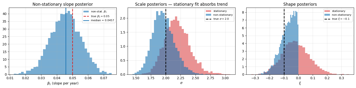

Reading these.

The non-stationary posterior on $\beta_1$ is concentrated around the planted slope 0.05 (median $\approx 0.046$ , 95% CI covering the truth) — the data clearly identifies the trend.
The stationary $\sigma$ posterior sits high relative to the true $\sigma = 2.0$ , while the non-stationary posterior recovers it: the stationary model has nowhere to put the trend except by inflating the implied dispersion.
The stationary $\xi$ posterior drifts toward zero (a heavier apparent tail): with the trend artificially smearing the maxima, the stationary model misreads the tail shape. The non-stationary fit (with its bounded-tail $\xi < 0$ prior) keeps $\xi$ closer to the true -0.10.

6. Time-varying return-level curve¶

Under non-stationarity the year- $T$ return level is itself a function of time:

z_T(t) \;=\; \mu(t) + \frac{\sigma}{\xi}\Bigl[(-\log(1 - 1/T))^{-\xi} - 1\Bigr] \;=\; (\beta_0 + \beta_1 t) + \frac{\sigma}{\xi}\bigl[\ldots\bigr].

(8)

We compute it from each posterior sample to get a 95% credible band — the entire excess part is stationary, the trend lives entirely in $\mu(t)$ .

T = 100.0


def excess_at_T(sigma, xi, T_):
    safe_xi = jnp.where(jnp.abs(xi) < 1e-7, 1.0, xi)
    return jnp.where(
        jnp.abs(xi) < 1e-7,
        -sigma * jnp.log(-jnp.log(1.0 - 1.0 / T_)),
        (sigma / safe_xi) * (jnp.power(-jnp.log(1.0 - 1.0 / T_), -safe_xi) - 1.0),
    )


excess_T_ns = jax.vmap(lambda s, x: excess_at_T(s, x, T))(
    posterior_ns["sigma"], posterior_ns["xi"]
)
excess_T_s = jax.vmap(lambda s, x: excess_at_T(s, x, T))(
    posterior_s["sigma"], posterior_s["xi"]
)

# Grid spans the full record: years 0 .. N_YEARS - 1 (the same span as the data).
t_grid = jnp.arange(0, N_YEARS, dtype=jnp.float32)
mu_grid = (
    posterior_ns["beta0"][:, None] + posterior_ns["beta1"][:, None] * t_grid[None, :]
)
zT_ns = mu_grid + excess_T_ns[:, None]
zT_s_const = posterior_s["mu"] + excess_T_s
zT_s = jnp.broadcast_to(zT_s_const[:, None], (zT_s_const.shape[0], t_grid.shape[0]))

zT_true = (BETA0_TRUE + BETA1_TRUE * np.asarray(t_grid)) + float(
    excess_at_T(jnp.array(SIGMA_TRUE), jnp.array(XI_TRUE), T)
)

fig, ax = plt.subplots(figsize=(10, 5))
ax.scatter(
    np.asarray(years),
    np.asarray(maxima),
    color="tab:gray",
    label="annual maxima",
    zorder=3,
)
ax.fill_between(
    np.asarray(t_grid),
    np.asarray(jnp.quantile(zT_ns, 0.025, axis=0)),
    np.asarray(jnp.quantile(zT_ns, 0.975, axis=0)),
    color="tab:blue",
    alpha=0.25,
    label="non-stat. 95% CI",
)
ax.plot(
    np.asarray(t_grid),
    np.asarray(jnp.median(zT_ns, axis=0)),
    color="tab:blue",
    lw=2,
    label=rf"non-stat. $z_{{T={T:.0f}}}(t)$",
)
ax.fill_between(
    np.asarray(t_grid),
    np.asarray(jnp.quantile(zT_s, 0.025, axis=0)),
    np.asarray(jnp.quantile(zT_s, 0.975, axis=0)),
    color="tab:red",
    alpha=0.2,
)
ax.plot(
    np.asarray(t_grid),
    np.asarray(jnp.median(zT_s, axis=0)),
    color="tab:red",
    lw=2,
    ls="--",
    label=rf"stationary $z_{{T={T:.0f}}}$",
)
ax.plot(np.asarray(t_grid), zT_true, color="black", lw=2, ls=":", label="true $z_T(t)$")
ax.set_xlabel("year (since 1945)")
ax.set_ylabel("level")
ax.set_title("100-year return level: stationary vs non-stationary fit")
ax.grid(True, alpha=0.3)
ax.legend(fontsize=8, loc="upper left")
plt.tight_layout()
plt.show()

t_first = float(t_grid[0])
t_last = float(t_grid[-1])
span = t_last - t_first  # actual interval spanned by the grid (years)
z_start = float(jnp.median(zT_ns[:, 0]))
z_end = float(jnp.median(zT_ns[:, -1]))
# Slope of the return-level curve over the ACTUAL span (it equals beta1 because
# the excess term is stationary): divide the endpoint rise by the span, not N_YEARS.
rl_slope = (z_end - z_start) / span
slope_med = float(jnp.median(posterior_ns["beta1"]))
slope_lo = float(jnp.quantile(posterior_ns["beta1"], 0.025))
slope_hi = float(jnp.quantile(posterior_ns["beta1"], 0.975))
print(f"Non-stat. 100-yr return level at year {t_first:.0f}:  {z_start:.2f}")
print(f"Non-stat. 100-yr return level at year {t_last:.0f}: {z_end:.2f}")
print(
    f"Return-level slope over years {t_first:.0f}-{t_last:.0f} "
    f"(span {span:.0f} yr):  {rl_slope:.4f}/yr"
)
print(
    f"Recovered slope (β1 posterior):           "
    f"{slope_med:.4f}/yr  [95% CI: {slope_lo:.4f}, {slope_hi:.4f}]"
)
print(f"True slope (β1):                          {BETA1_TRUE:.4f}/yr")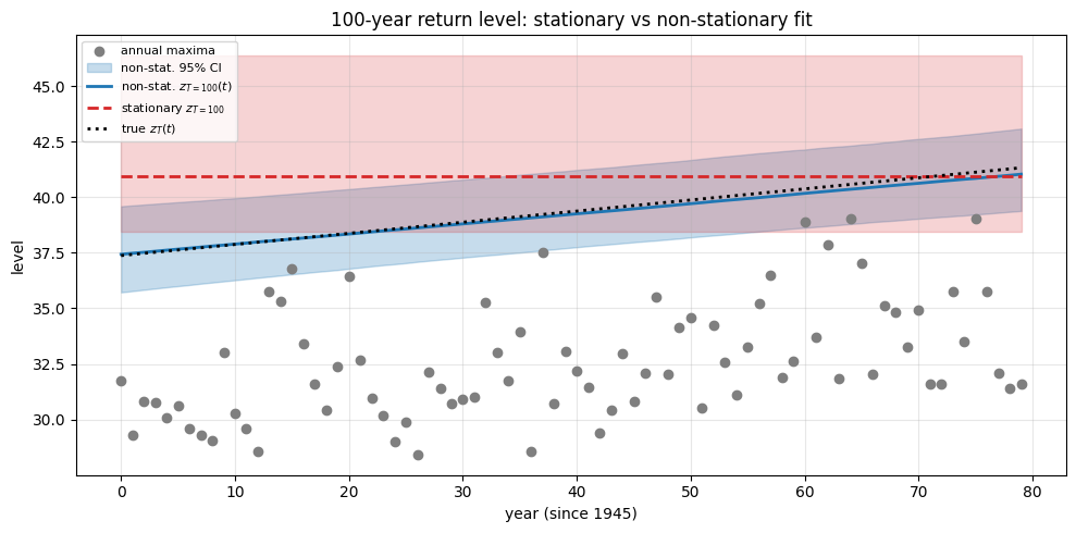

Non-stat. 100-yr return level at year 0:  37.43
Non-stat. 100-yr return level at year 79: 41.03
Return-level slope over years 0-79 (span 79 yr):  0.0456/yr
Recovered slope (β1 posterior):           0.0457/yr  [95% CI: 0.0262, 0.0643]
True slope (β1):                          0.0500/yr

The picture is unambiguous. The non-stationary fit produces a return-level curve that rises in lockstep with the trend; the stationary fit produces a flat line that under-predicts late-record extremes and over-predicts early-record extremes. Both are wrong by the same total amount, but the non-stationary fit puts the error in the right place (the trend term) while the stationary fit smears it across $\sigma$ and $\xi$ .

7. Posterior predictive check¶

A quick sanity check: simulate a replicate dataset from the non-stationary posterior and compare to the data.

n_post = 200
idx = jax.random.choice(KEY, len(posterior_ns["beta0"]), shape=(n_post,), replace=False)


def sample_replicate(key, b0, b1, sigma, xi):
    mu_t = b0 + b1 * years
    return GeneralizedExtremeValueDistribution(
        loc=mu_t, scale=sigma, concentration=xi
    ).sample(key)


keys = jax.random.split(KEY, n_post)
replicates = jax.vmap(sample_replicate)(
    keys,
    posterior_ns["beta0"][idx],
    posterior_ns["beta1"][idx],
    posterior_ns["sigma"][idx],
    posterior_ns["xi"][idx],
)

fig, ax = plt.subplots(figsize=(10, 4))
for r in np.asarray(replicates)[::10]:
    ax.plot(np.asarray(years), r, color="tab:blue", lw=0.5, alpha=0.2)
ax.scatter(
    np.asarray(years),
    np.asarray(maxima),
    color="tab:red",
    zorder=3,
    s=20,
    label="observed",
)
ax.plot(
    np.asarray(years),
    np.asarray(jnp.median(replicates, axis=0)),
    color="tab:blue",
    lw=2,
    label="posterior predictive median",
)
ax.set_xlabel("year (since 1945)")
ax.set_ylabel("annual maximum")
ax.set_title("Posterior predictive simulations")
ax.grid(True, alpha=0.3)
ax.legend()
plt.tight_layout()
plt.show()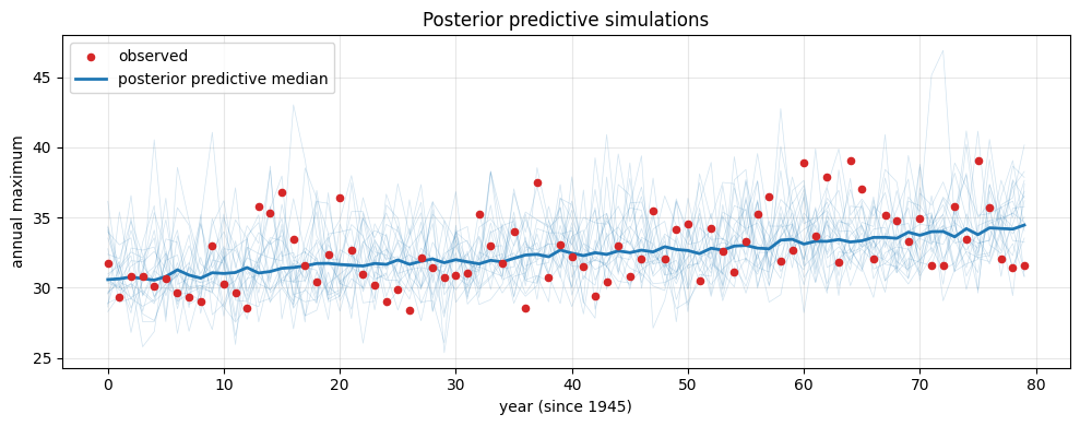

Takeaways¶

Non-stationarity in $\mu$ is the simplest and most useful covariate-driven extension of the GEVD. A linear-in-time $\mu(t) = \beta_0 + \beta_1 t$ adds a single parameter and dramatically reduces bias.
Stationary mis-specification is recoverable in $\sigma$ . Under a planted trend, the stationary fit inflates $\sigma$ to absorb the trend variance — a tell-tale sign that you should be fitting non-stationary.
Return levels translate. With $\mu(t)$ linear and $(\sigma, \xi)$ fixed, $z_T(t)$ is also linear and its slope equals $\beta_1$ — independent of $T$ .
Don’t make $\xi$ non-stationary unless forced. In real datasets $\xi$ is already poorly identified; a covariate-dependent $\xi$ blows up the posterior.
Generalisation. Replace the linear basis $(1, t)$ with $(1, t, z_t)$ to add a covariate, or with a polynomial / spline basis for non-linear trends. The next two notebooks in this mini-series do exactly that — non-parametric splines and ODE-driven dynamics — but the idea is the same: pick a parameterisation of $\mu(\cdot)$ rich enough for the trend, leave $(\sigma, \xi)$ stationary, and fit.