Inhomogeneous Poisson Process — From Scratch and With NumPyro

The inhomogeneous Poisson process (IPP) generalises the HPP by letting the intensity $\lambda(t)$ vary in time. The compensator $\Lambda(t) = \int_0^t \lambda(s)\, ds$ replaces the linear $\lambda t$ , and the log-likelihood becomes

\log L\bigl(\{t_i\}_{i=1}^n\bigr) = \sum_{i=1}^n \log \lambda(t_i) \;-\; \Lambda(T).

(1)

This notebook shows both sides of the xtremax stack:

From scratch — call the pure primitives directly: Lewis–Shedler thinning to sample, ipp_log_prob to evaluate the likelihood, time-rescaling residuals for a goodness-of-fit check.
With NumPyro — wrap the IPP as a numpyro.distributions.Distribution and run NUTS over the log-rates of a piecewise-constant intensity.

Setup¶

%pip install -q xtremax matplotlib  # uncomment on Colab
import jax
import jax.numpy as jnp
import matplotlib.pyplot as plt
import numpy as np
import numpyro
import numpyro.distributions as dist
from jax import random
from numpyro.infer import MCMC, NUTS

from xtremax.point_processes.distributions import (
    InhomogeneousPoissonProcess as IppDist,
)
from xtremax.point_processes.operators import PiecewiseConstantLogIntensity
from xtremax.point_processes.primitives import (
    ipp_log_prob,
    ipp_sample_thinning,
    ks_statistic_exp1,
    qq_exp1_quantiles,
    time_rescaling_residuals,
)


plt.rcParams["figure.figsize"] = (8.0, 3.5)

/home/azureuser/localfiles/xtremax/.venv/bin/python: No module named pip

Note: you may need to restart the kernel to use updated packages.

/home/azureuser/localfiles/xtremax/.venv/lib/python3.13/site-packages/tqdm/auto.py:21: TqdmWarning: IProgress not found. Please update jupyter and ipywidgets. See https://ipywidgets.readthedocs.io/en/stable/user_install.html
  from .autonotebook import tqdm as notebook_tqdm

1. From scratch — the primitives layer¶

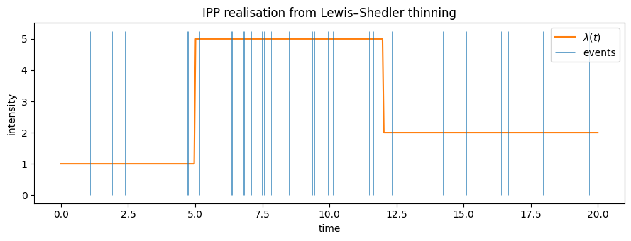
Pick a piecewise-constant log-intensity. Three bins, three rates. PiecewiseConstantLogIntensity is an eqx.Module that stores bin_edges and log_rates as PyTree leaves; for our purposes here we just need two things from it: it’s a callable log_intensity_fn(t) that returns $\log \lambda(t)$ , and it has a closed-form .integrate(a, b) that returns $\int_a^b \lambda(s)\, ds$ exactly.

true_bin_edges = jnp.array([0.0, 5.0, 12.0, 20.0])
true_rates = jnp.array([1.0, 5.0, 2.0])
true_intensity = PiecewiseConstantLogIntensity(
    bin_edges=true_bin_edges, rates=true_rates
)

T = float(true_bin_edges[-1])
true_Lambda_T = true_intensity.integrate(0.0, T)
true_lambda_max = true_intensity.max_intensity()
print(f"Λ(T) (closed form)   = {float(true_Lambda_T):.3f}")
print(f"λ_max (closed form)  = {float(true_lambda_max):.3f}")

Λ(T) (closed form)   = 56.000
λ_max (closed form)  = 5.000

Sampling via Lewis–Shedler thinning¶

The ipp_sample_thinning primitive oversamples from a homogeneous process at rate $\lambda_{\max}$ and accepts each candidate with probability $\lambda(t) / \lambda_{\max}$ . It returns (times, mask, n_candidates_uncapped) on a static buffer so the routine stays jit-compatible.

times, mask, n_cand = ipp_sample_thinning(
    key=random.PRNGKey(0),
    log_intensity_fn=true_intensity,
    T=T,
    lambda_max=true_lambda_max,
    max_candidates=256,
)
print(f"Accepted {int(mask.sum())} events out of {int(n_cand)} candidates")

fig, ax = plt.subplots(figsize=(9, 3.5))
grid = np.linspace(0, T, 400)
ax.plot(
    grid,
    np.asarray(jnp.exp(true_intensity(jnp.asarray(grid)))),
    color="C1",
    label=r"$\lambda(t)$",
)
ax.vlines(
    np.asarray(times[mask]),
    0,
    float(true_lambda_max) * 1.05,
    color="C0",
    linewidth=0.6,
    alpha=0.8,
    label="events",
)
ax.set_xlabel("time")
ax.set_ylabel("intensity")
ax.set_title("IPP realisation from Lewis–Shedler thinning")
ax.legend()
plt.tight_layout()
plt.show()

Accepted 42 events out of 85 candidates

Evaluating the log-likelihood¶

ipp_log_prob(event_times, mask, log_intensity_fn, integrated_intensity) returns $\sum_i \log \lambda(t_i) - \Lambda(T)$ . We can compute $\Lambda(T)$ once via the closed-form .integrate method and reuse it.

Lambda_T = true_intensity.integrate(0.0, T)
log_L = ipp_log_prob(times, mask, true_intensity, Lambda_T)
print(f"log L at the true intensity: {float(log_L):.3f}")

log L at the true intensity: -8.139

Goodness-of-fit via the time-rescaling theorem¶

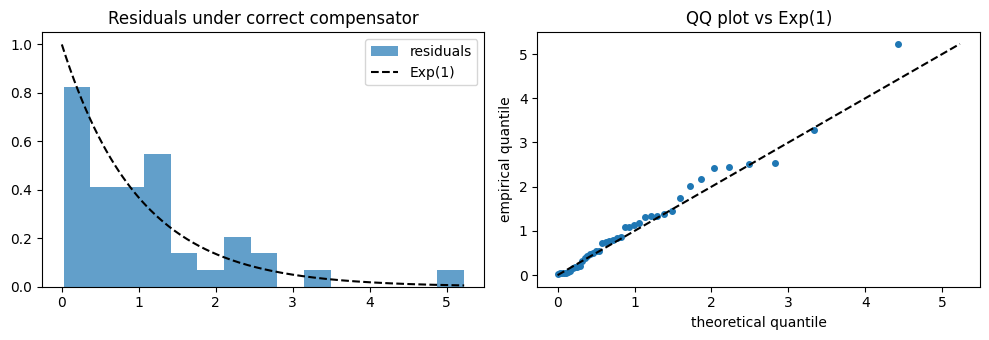
Under the time-rescaling theorem, if $\Lambda$ is the correct compensator of the process, the rescaled inter-event times $\tau_i = \Lambda(t_i) - \Lambda(t_{i-1})$ are i.i.d. $\mathrm{Exp}(1)$ . Plugging the compensator into time_rescaling_residuals and then through ks_statistic_exp1 gives a one-line goodness-of-fit check that works for any point-process model with a well-defined compensator.

def Lambda_correct(t):
    # Vectorised over a batched ``t`` using the module's closed form.
    flat_t = jnp.atleast_1d(jnp.asarray(t))
    zeros = jnp.zeros_like(flat_t)
    return jax.vmap(true_intensity.integrate)(zeros, flat_t).reshape(jnp.shape(t))


residuals, res_mask = time_rescaling_residuals(times, mask, Lambda_correct)
ks = ks_statistic_exp1(residuals, res_mask)
theo, emp = qq_exp1_quantiles(residuals, res_mask)
print(f"KS statistic (correct compensator) : {float(ks):.3f}")


# Wrong compensator — pretend the process is HPP with λ=1.
def Lambda_wrong(t):
    return jnp.asarray(t)


res_w, _ = time_rescaling_residuals(times, mask, Lambda_wrong)
ks_w = ks_statistic_exp1(res_w, res_mask)
print(f"KS statistic (wrong λ≡1)          : {float(ks_w):.3f}")

fig, (ax0, ax1) = plt.subplots(1, 2, figsize=(10, 3.5))

real_res = np.asarray(residuals[res_mask])
ax0.hist(real_res, bins=15, density=True, alpha=0.7, color="C0", label="residuals")
xx = np.linspace(0, real_res.max(), 200)
ax0.plot(xx, np.exp(-xx), "k--", label=r"Exp(1)")
ax0.legend()
ax0.set_title("Residuals under correct compensator")

theo_np = np.asarray(theo)
emp_np = np.asarray(emp)
good = ~np.isnan(theo_np)
ax1.plot(theo_np[good], emp_np[good], "o", color="C0", markersize=4)
lim = max(theo_np[good].max(), emp_np[good].max())
ax1.plot([0, lim], [0, lim], "k--")
ax1.set_xlabel("theoretical quantile")
ax1.set_ylabel("empirical quantile")
ax1.set_title("QQ plot vs Exp(1)")
plt.tight_layout()
plt.show()

KS statistic (correct compensator) : 0.089
KS statistic (wrong λ≡1)          : 0.462

2. With NumPyro — Bayesian inference over log-rates¶

To recover the bin rates from the event sequence we put a prior on the per-bin log-rates and run NUTS. The IPP likelihood is IppDist(...).log_prob((times, mask)), evaluated with a freshly-constructed intensity at each MCMC step.

The operator (and therefore the distribution wrapper) queries $\Lambda(T)$ from the current intensity module on every log_prob call, so the $-\Lambda(T)$ term tracks updated log-rates automatically — crucial for Bayesian inference and for any gradient-based downstream use.

def bayesian_model(times, mask, bin_edges):
    n_bins = bin_edges.shape[0] - 1
    log_rates = numpyro.sample(
        "log_rates",
        dist.Normal(jnp.zeros(n_bins), 2.0 * jnp.ones(n_bins)),
    )
    intensity_fn = PiecewiseConstantLogIntensity(
        bin_edges=bin_edges, log_rates=log_rates
    )
    ipp = IppDist(
        log_intensity_fn=intensity_fn,
        observation_window=bin_edges[-1],
        max_candidates=256,
    )
    numpyro.factor("lik", ipp.log_prob((times, mask)))


mcmc = MCMC(
    NUTS(bayesian_model),
    num_warmup=500,
    num_samples=1000,
    progress_bar=False,
)
mcmc.run(random.PRNGKey(0), times=times, mask=mask, bin_edges=true_bin_edges)
samples = mcmc.get_samples()
rate_samples = np.exp(np.asarray(samples["log_rates"]))

print("Posterior summary (rates):")
for b in range(true_rates.shape[0]):
    mean = rate_samples[:, b].mean()
    lo = np.quantile(rate_samples[:, b], 0.025)
    hi = np.quantile(rate_samples[:, b], 0.975)
    print(
        f"  bin {b}: mean {mean:.2f}, 95% CI [{lo:.2f}, {hi:.2f}], "
        f"true {float(true_rates[b]):.2f}"
    )

Posterior summary (rates):
  bin 0: mean 1.20, 95% CI [0.44, 2.28], true 1.00
  bin 1: mean 3.53, 95% CI [2.29, 5.06], true 5.00
  bin 2: mean 1.36, 95% CI [0.66, 2.32], true 2.00

fig, axes = plt.subplots(1, true_rates.shape[0], figsize=(11, 3.2), sharey=True)
for b, ax in enumerate(axes):
    ax.hist(rate_samples[:, b], bins=40, density=True, alpha=0.7, color="C0")
    ax.axvline(float(true_rates[b]), color="k", linestyle="--", label="true")
    ax.set_title(f"bin {b}")
    ax.set_xlabel(r"$\lambda$")
    if b == 0:
        ax.set_ylabel("density")
        ax.legend()
plt.tight_layout()
plt.show()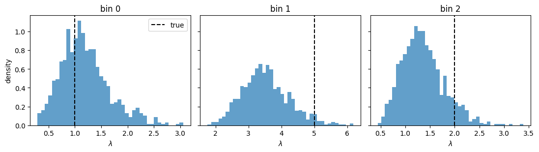

Posterior predictive check¶

Draw per-bin rate vectors from the posterior, simulate new event sequences, and compare the mean intensity profile with the truth. (We hold the bin edges fixed; the uncertainty is entirely on the rates.)

def simulate_once(key, log_rates):
    intensity = PiecewiseConstantLogIntensity(
        bin_edges=true_bin_edges, log_rates=log_rates
    )
    lam_max = intensity.max_intensity()
    ts, msk, _ = ipp_sample_thinning(key, intensity, T, lam_max, max_candidates=256)
    return ts, msk


keys_pp = random.split(random.PRNGKey(3), 200)
log_rates_pp = jnp.asarray(samples["log_rates"][:200])
ts_pp, msk_pp = jax.vmap(simulate_once)(keys_pp, log_rates_pp)

# Histogram events across posterior-predictive draws.
all_times = np.asarray(ts_pp)[np.asarray(msk_pp)]
fig, ax = plt.subplots(figsize=(9, 3.5))
ax.hist(
    all_times,
    bins=40,
    density=True,
    alpha=0.7,
    color="C0",
    label="posterior predictive",
)
grid = np.linspace(0, T, 400)
ax.plot(
    grid,
    np.asarray(jnp.exp(true_intensity(jnp.asarray(grid)))) / float(true_Lambda_T),
    "k--",
    label=r"true $\lambda(t) / \Lambda(T)$",
)
ax.set_xlabel("time")
ax.set_ylabel("event density")
ax.set_title("Posterior-predictive event density")
ax.legend()
plt.tight_layout()
plt.show()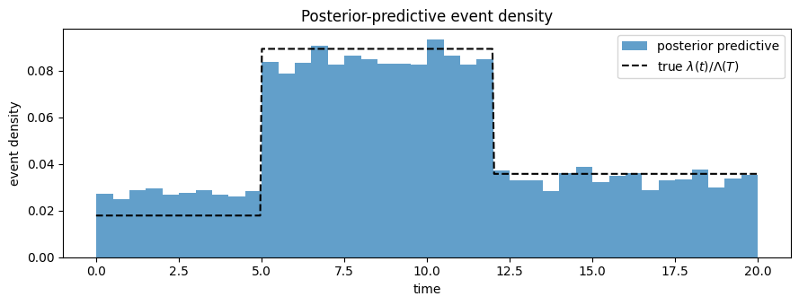

Takeaways¶

Primitives are enough to sample, evaluate the likelihood, and run time-rescaling goodness-of-fit for any intensity $\lambda(t)$ — no operator or distribution required.
PiecewiseConstantLogIntensity is the natural parameterisation for piecewise-constant rates: its log_rates leaf is both a plain eqx.Module parameter (jit/vmap/grad friendly) and a NumPyro-friendly field (samplable via numpyro.sample).
The operator’s .log_prob always computes $\Lambda(T)$ from the live intensity, so posteriors from NUTS (or any gradient-based optimiser) see the full likelihood — the $\sum \log \lambda(t_i)$ term and the $-\Lambda(T)$ term — rather than a stale cache.