Independent fits, fast — a Laplace approximation

Abstract¶

Notebook 04 fit every station independently with NUTS — honest, but on the full century-long Iberian record (107 stations, ragged) a single fit takes minutes, and it needed careful reparameterising just to stop the sampler diverging. Here we fit the same no-pooling model with a Laplace approximation: optimise to the posterior mode and read the covariance off the curvature there. It returns in seconds, and lands on the same maps and the same signal-to-noise verdict — location μ(s) is real geography, the tail ξ(s) is mostly noise. Laplace is the workhorse we lean on for the heavier pooled and spatial models that follow; this notebook calibrates it against the NUTS baseline of notebook 04.

Keywords:Laplace approximationno poolingGEVmasked likelihoodreturn levels¶

Independent fits, fast: a Laplace approximation¶

Notebook 04 established the no-pooling baseline — one GEV per station, fit jointly with NUTS — and its verdict: the location $\mu(s)$ is smooth and real, while the scale and especially the tail $\xi(s)$ are dominated by sampling noise. It also cost a few minutes per fit on the full record and needed a careful $\log\sigma$ / bounded- $\xi$ reparameterisation to keep the sampler off the GEV’s support edge.

For everything from here on we switch the workhorse inference to a Laplace approximation: find the posterior mode (the MAP) by optimisation, then approximate the posterior by the Gaussian whose covariance is the inverse Hessian at that mode. One optimisation, a few seconds, and — when the posterior is roughly Gaussian — an answer that matches full MCMC. This notebook fits the exact same no-pooling model that way and checks it lands where notebook 04’s NUTS run did.

The model is unchanged: per-station $\mu_s$ , $\log\sigma_s$ and $\xi_s = \tfrac12\tanh\tilde\xi_s$ , with the likelihood masked over the ragged records (each station is seen in a different subset of the 1897–2025 years).

import sys
import pathlib

try:
    import spatial_extremes  # noqa: F401  already importable (e.g. on PYTHONPATH)
except ModuleNotFoundError:
    _here = pathlib.Path.cwd().resolve()
    _roots = (_here, *_here.parents)
    _cands = [r / "_helpers" for r in _roots]
    _cands += [r / "docs" / "tutorials" / "spatial_extremes" / "_helpers" for r in _roots]
    _src = next((c for c in _cands if (c / "spatial_extremes").exists()), None)
    if _src is None:
        raise RuntimeError("cannot locate docs/tutorials/spatial_extremes/_helpers") from None
    sys.path.insert(0, str(_src))

import jax
jax.config.update("jax_enable_x64", True)

import time

import numpy as np
import jax
import jax.numpy as jnp
import jax.random as jr
import optax
import matplotlib.pyplot as plt

import numpyro
import numpyro.distributions as ndist
from numpyro.infer import SVI, Trace_ELBO, Predictive
from numpyro.infer.autoguide import AutoLaplaceApproximation
from numpyro.infer.initialization import init_to_median

from xtremax import GeneralizedExtremeValueDistribution as GEV
from spatial_extremes import data
from spatial_extremes.viz import iberia_axes, scatter_field

maxima, stations, years, is_real = data.load_annual_maxima(min_years=20)
Y = jnp.asarray(maxima)              # (S, T) — NaN where a station-year is missing
mask = ~jnp.isnan(Y)
lon, lat = stations[:, 0], stations[:, 1]
S, T = Y.shape
ybar = jnp.asarray(np.nanmean(maxima, axis=1))
ystd = jnp.asarray(np.nanstd(maxima, axis=1))
n_obs = np.asarray(mask.sum(1))
print("source:", "REAL" if is_real else "SYNTHETIC",
      "| stations", S, "| years", f"{years.min()}-{years.max()}", f"({T})")
print(f"coverage: {int(n_obs.min())}-{int(n_obs.max())} yrs/station, "
      f"{100 * float(mask.mean()):.0f}% of the {S}×{T} grid observed")

source: REAL | stations 107 | years 1897-2025 (125)
coverage: 23-120 yrs/station, 49% of the 107×125 grid observed

The model and the Laplace fit¶

Same no-pooling model as notebook 04 — fixed per-station priors, no parameter shared across stations — with the stabilising $\log\sigma$ / bounded- $\xi$ reparameterisation and a masked likelihood that sums $\log p(y_{s,t})$ only over observed station-years (gaps filled with an in-support value and zeroed out via numpyro.factor).

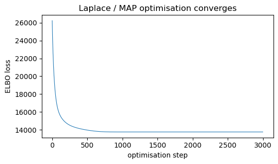
AutoLaplaceApproximation optimises this to its MAP and reads the Gaussian posterior off the curvature. We drive it with Adam (guarding the occasional out-of-support GEV gradient); the ELBO loss should settle onto a flat plateau — the sign it has found the mode.

def gev_no_pool(Y):
    with numpyro.plate("stations", S):
        mu = numpyro.sample("mu", ndist.Normal(ybar, 5.0))
        log_sigma = numpyro.sample("log_sigma", ndist.Normal(jnp.log(ystd), 0.5))
        xi_t = numpyro.sample("xi_t", ndist.Normal(0.0, 0.5))
        sigma = numpyro.deterministic("sigma", jnp.exp(log_sigma))
        xi = numpyro.deterministic("xi", 0.5 * jnp.tanh(xi_t))
    # masked likelihood: only observed (non-NaN) station-years contribute
    yf = jnp.where(mask, Y, ybar[:, None])
    lp = GEV(loc=mu[:, None], scale=sigma[:, None],
             concentration=xi[:, None]).log_prob(yf)
    numpyro.factor("obs", jnp.where(mask, lp, 0.0).sum())

guide = AutoLaplaceApproximation(gev_no_pool, init_loc_fn=init_to_median)
opt = numpyro.optim.optax_to_numpyro(
    optax.chain(optax.zero_nans(), optax.clip_by_global_norm(10.0), optax.adam(3e-3))
)
svi = SVI(gev_no_pool, guide, opt, Trace_ELBO())
t0 = time.time()
res = svi.run(jr.PRNGKey(0), 3000, Y, progress_bar=False)
print(f"Laplace fit {S} stations in {time.time() - t0:.1f}s "
      f"(NUTS in notebook 04 took several minutes)")

fig, ax = plt.subplots(figsize=(6, 3.2))
ax.plot(np.asarray(res.losses), lw=0.8)
ax.set_xlabel("optimisation step")
ax.set_ylabel("ELBO loss")
ax.set_title("Laplace / MAP optimisation converges")
plt.show()

Laplace fit 107 stations in 2.9s (NUTS in notebook 04 took several minutes)

Read off the posterior¶

Draw from the Laplace Gaussian with guide.sample_posterior, then push the draws through Predictive to get posterior samples of $\mu, \sigma, \xi$ per station.

lap = guide.sample_posterior(jr.PRNGKey(1), res.params, sample_shape=(800,))
pred = Predictive(gev_no_pool, posterior_samples=lap,
                  return_sites=["mu", "sigma", "xi"])(jr.PRNGKey(2), Y)

def summarise(name):
    a = np.asarray(pred[name])
    return (np.median(a, 0),
            np.quantile(a, 0.025, 0),
            np.quantile(a, 0.975, 0))

mu_med, mu_lo, mu_hi = summarise("mu")
sig_med, sig_lo, sig_hi = summarise("sigma")
xi_med, xi_lo, xi_hi = summarise("xi")
print("μ  median range:", mu_med.round(1).min(), "->", mu_med.round(1).max(), "°C")
print("σ  median range:", sig_med.round(2).min(), "->", sig_med.round(2).max(), "°C")
print("ξ  median range:", xi_med.round(2).min(), "->", xi_med.round(2).max())

μ  median range: 21.3 -> 42.3 °C
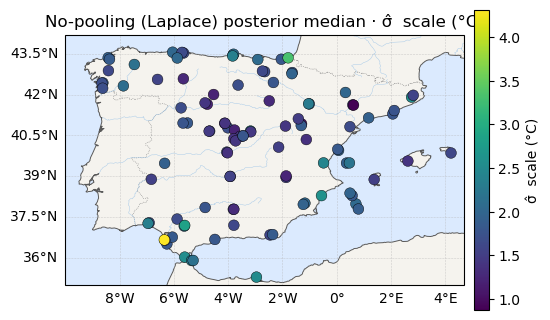
σ  median range: 0.88 -> 4.31 °C
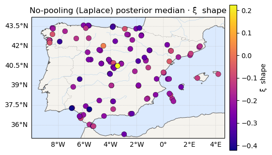
ξ  median range: -0.42 -> 0.22

The maps¶

Posterior-median $\mu$ , $\sigma$ , $\xi$ — location on a temperature scale, scale on viridis, shape on plasma. As in notebook 04, $\mu$ reads as a map and $\xi$ reads as static.

for vals, label, cmap in [(mu_med, "μ̂  location (°C)", "RdYlBu_r"),
                          (sig_med, "σ̂  scale (°C)", "viridis"),
                          (xi_med, "ξ̂  shape", "plasma")]:
    ax = iberia_axes(figsize=(6.2, 5.2))
    scatter_field(ax, lon, lat, vals, label=label, cmap=cmap)
    ax.set_title(f"No-pooling (Laplace) posterior median · {label}")
    plt.show()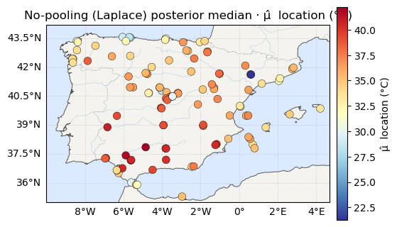

The same signal-to-noise verdict¶

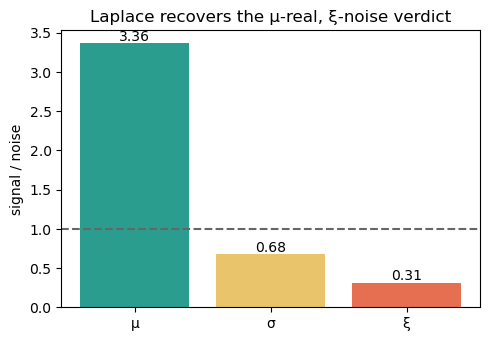
The diagnostic from notebook 04: for each parameter, the spread of the point estimates across stations (signal) over the typical within-station 95% credible-interval width (noise). Above 1, the map is real; below 1, it is mostly sampling noise. Laplace should reproduce notebook 04’s ordering — $\mu$ well above the floor, $\xi$ well below.

rows = []
for name, (med, lo, hi) in [("μ", (mu_med, mu_lo, mu_hi)),
                            ("σ", (sig_med, sig_lo, sig_hi)),
                            ("ξ", (xi_med, xi_lo, xi_hi))]:
    signal, noise = med.std(), (hi - lo).mean()
    rows.append((name, signal / noise))
    print(f"{name}:  signal SD(med)={signal:6.3f}   noise mean-CI-width={noise:6.3f}"
          f"   ratio={signal / noise:5.2f}")

fig, ax = plt.subplots(figsize=(5.4, 3.6))
names = [r[0] for r in rows]
ratios = [r[1] for r in rows]
bars = ax.bar(names, ratios, color=["#2a9d8f", "#e9c46a", "#e76f51"])
ax.axhline(1.0, ls="--", color="0.4")
ax.set_ylabel("signal / noise")
ax.set_title("Laplace recovers the μ-real, ξ-noise verdict")
for b, r in zip(bars, ratios):
    ax.text(b.get_x() + b.get_width() / 2, r + 0.03, f"{r:.2f}", ha="center")
plt.show()

μ:  signal SD(med)= 3.403   noise mean-CI-width= 1.011   ratio= 3.36
σ:  signal SD(med)= 0.455   noise mean-CI-width= 0.670   ratio= 0.68
ξ:  signal SD(med)= 0.096   noise mean-CI-width= 0.306   ratio= 0.31

Return levels¶

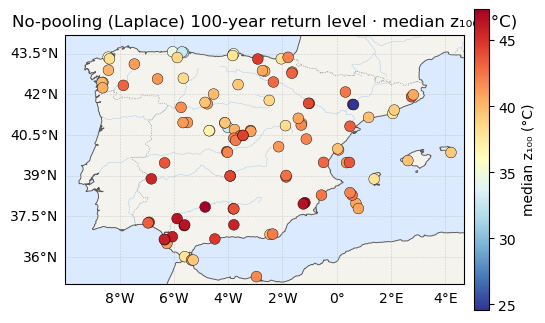
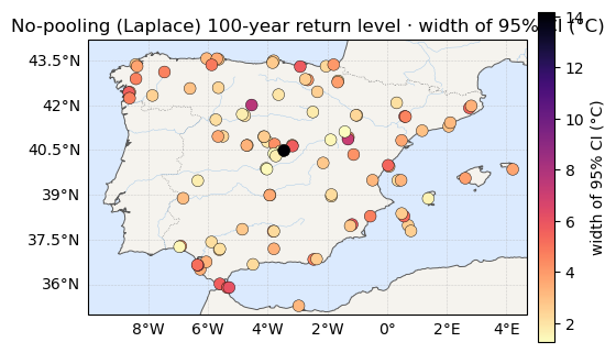
The 100-year level at every station, with its 95% credible band — the planner-facing summary, now in seconds.

RL = GEV(loc=jnp.asarray(pred["mu"]), scale=jnp.asarray(pred["sigma"]),
         concentration=jnp.asarray(pred["xi"])).return_level(100.0)  # (n, S)
RL = np.asarray(RL)
rl_med = np.median(RL, 0)
rl_ciw = np.quantile(RL, 0.975, 0) - np.quantile(RL, 0.025, 0)
print(f"z100 median range: {rl_med.min():.1f} -> {rl_med.max():.1f} °C")
print(f"z100 95% CI width: {rl_ciw.mean():.1f} °C avg (up to {rl_ciw.max():.1f})")

for vals, label, cmap in [(rl_med, "median z₁₀₀ (°C)", "RdYlBu_r"),
                          (rl_ciw, "width of 95% CI (°C)", "magma_r")]:
    ax = iberia_axes(figsize=(6.2, 5.2))
    scatter_field(ax, lon, lat, vals, label=label, cmap=cmap)
    ax.set_title(f"No-pooling (Laplace) 100-year return level · {label}")
    plt.show()

z100 median range: 24.6 -> 47.3 °C
z100 95% CI width: 3.4 °C avg (up to 14.2)

Takeaway¶

Same model, same data, same conclusion as notebook 04 — $\mu$ is real geography, $\xi$ is noise — but in seconds rather than minutes, and with no divergences to wrestle (Laplace optimises; it does not sample). That speed is what makes the pooled and spatial models in the rest of the curriculum practical on the full century-long record.

The one caveat, as always with Laplace: a Gaussian at the mode can mis-state interval widths when the true posterior is skewed — most acutely for the tail. Where the calibrated uncertainty is the deliverable, it is worth a confirmatory NUTS run (as in notebook 04, and the spatial notebooks’ Laplace-vs-NUTS checks). For mapping and model-building, Laplace is the right default.