Three fields — a fully non-stationary GEV

Abstract¶

The last step of the spatial build-up: every GEV parameter becomes its own Gaussian-process field. On top of the location μ(s) and scale σ(s) of notebook 08, the shape ξ(s) — the tail exponent — gets a third GP. The model is fully non-stationary, and fits with the same mean-field variational approximation as notebook 08. The point is as much diagnostic as predictive: ξ is barely identifiable even pooled globally (notebook 04), so we ask honestly whether a spatial prior can recover any tail geography, or whether the ξ(s) field just reproduces per-station noise. The answer shapes how far non-stationarity is worth pushing.

Keywords:non-stationary extremesGaussian processspatial shape parameteridentifiabilityvariational inference¶

Three fields: a fully non-stationary spatial GEV¶

Notebook 07 made the location spatial; notebook 08 added a spatial scale. The only parameter still forced to a single global value is the shape $\xi$ — the tail exponent that decides whether extremes are bounded ( $\xi<0$ ), light ( $\xi=0$ ) or heavy ( $\xi>0$ ). This notebook frees it too, giving the GEV a third Gaussian-process field and making it fully non-stationary:

y_{s,t} \sim \mathrm{GEV}\big(\mu(s),\ \sigma(s),\ \xi(s)\big),

(1)

\begin{aligned} \mu(s) &= \mu_0 + f_\mu(s) + \varepsilon^\mu_s, \\ \log\sigma(s) &= \lambda_0 + f_\sigma(s) + \varepsilon^\sigma_s, \\ \tilde\xi(s) &= \xi_0 + f_\xi(s) + \varepsilon^\xi_s, \qquad \xi(s) = \tfrac12\tanh\tilde\xi(s), \end{aligned}

(2)

with three independent Matérn-3/2 GP fields, each with a fixed regional lengthscale and a fixed amplitude, plus per-station nuggets. The $\tfrac12\tanh$ keeps $\xi(s)$ in the stable, finite-mean band $(-\tfrac12, \tfrac12)$ from notebook 04.

This is the natural end of the build-up — but more parameters is not the same as more knowledge. Notebook 04 showed $\xi$ is dominated by sampling noise even when estimated per station, and notebook 05 showed a hierarchy pools it almost to a constant. So the real question here is diagnostic: given a free spatial field, does $\xi(s)$ discover any tail geography, or does it just paint the old per-station noise onto a map? We give $f_\xi$ a deliberately small prior amplitude — the honest prior is that the tail barely varies — and look.

import sys
import pathlib

try:
    import spatial_extremes  # noqa: F401  already importable (e.g. on PYTHONPATH)
except ModuleNotFoundError:
    _here = pathlib.Path.cwd().resolve()
    _roots = (_here, *_here.parents)
    _cands = [r / "_helpers" for r in _roots]
    _cands += [r / "docs" / "tutorials" / "spatial_extremes" / "_helpers" for r in _roots]
    _src = next((c for c in _cands if (c / "spatial_extremes").exists()), None)
    if _src is None:
        raise RuntimeError("cannot locate docs/tutorials/spatial_extremes/_helpers") from None
    sys.path.insert(0, str(_src))

import jax
jax.config.update("jax_enable_x64", True)

import time

import numpy as np
import jax
import jax.numpy as jnp
import jax.random as jr
import optax
import matplotlib.pyplot as plt

import numpyro
import numpyro.distributions as ndist
from numpyro.infer import SVI, Trace_ELBO, Predictive, MCMC, NUTS
from numpyro.infer.autoguide import AutoLaplaceApproximation, AutoNormal
from numpyro.infer.initialization import init_to_median

from pyrox.gp import GPPrior, Matern, gp_sample
from xtremax import GeneralizedExtremeValueDistribution as GEV
from xtremax import gev_return_level
from spatial_extremes import data
from spatial_extremes.viz import iberia_axes, scatter_field

maxima, stations, years, is_real = data.load_annual_maxima(min_years=20)
Y = jnp.asarray(maxima)                       # (S, T) — NaN where a year is missing
mask = ~jnp.isnan(Y)
S, T = Y.shape
lon, lat = stations[:, 0], stations[:, 1]
Xs = jnp.asarray(stations)
Xm, Xsd = Xs.mean(0), Xs.std(0)
Xn = (Xs - Xm) / Xsd                          # standardised coords for the kernel
ybar = jnp.asarray(np.nanmean(maxima, axis=1))
Y_MEAN = float(np.nanmean(maxima))
LENGTHSCALE = 0.8                             # fixed regional lengthscale (std units)
print("source:", "REAL" if is_real else "SYNTHETIC",
      "| stations", S, "| years", f"{years.min()}-{years.max()}", f"({T})")

# physical covariates for the scale field (derived in notebook 06),
# standardised so each coefficient is the log-σ change per 1 SD of the feature
from spatial_extremes.features import load_station_features

_feat = load_station_features(stations)
COV_COLS = ["elevation", "dist_coast_km"]
COV_LABELS = ["elevation", "dist-to-coast"]
_C = _feat[COV_COLS].to_numpy()
C = jnp.asarray((_C - _C.mean(0)) / _C.std(0))   # (S, n_cov)

/Users/eman/code_projects/research_notebook/projects/spatial_extremes/.venv/lib/python3.12/site-packages/tqdm/auto.py:21: TqdmWarning: IProgress not found. Please update jupyter and ipywidgets. See https://ipywidgets.readthedocs.io/en/stable/user_install.html
  from .autonotebook import tqdm as notebook_tqdm

source: REAL | stations 107 | years 1897-2025 (125)

The three-field model¶

The same gp_field helper as notebook 08, now called three times — each GP again uses a fixed lengthscale and amplitude (notebook 08 explains why a free amplitude is only weakly identified and destabilises the fit). The fixed amplitudes say how far we let each parameter roam: a few °C for the location, ~20% (in log units) for the scale, and a deliberately tight band for the shape — its honest setting is “nearly constant”, so the data must work hard to move it.

As in notebook 08, the scale also carries a linear covariate trend in elevation and distance-to-coast, $\log\sigma(s) = \lambda_0 + \beta^\top c(s) + f_\sigma(s) + \varepsilon^\sigma_s$ — 08 showed elevation (not raw coordinates) is what the regional scale structure was really tracking, so we keep it here too.

def gp_field(name, var, Xn):
    """A centred, whitened Matérn-3/2 GP with fixed lengthscale and amplitude."""
    k = Matern(pyrox_name="k_" + name, nu=1.5,
               init_lengthscale=LENGTHSCALE, init_variance=var)
    f = gp_sample("f_" + name, GPPrior(kernel=k, X=Xn), whitened=True)
    return f - jnp.mean(f)

def model(Xn, Y=None):
    f_mu = gp_field("mu", 4.0, Xn)            # location field (°C)
    f_ls = gp_field("ls", 0.1, Xn)            # log-scale field (log units)
    f_xi = gp_field("xi", 0.05, Xn)           # shape field (tanh pre-image)

    mu0 = numpyro.sample("mu0", ndist.Normal(Y_MEAN, 5.0))
    lam0 = numpyro.sample("lam0", ndist.Normal(jnp.log(2.0), 0.4))
    beta_ls = numpyro.sample(
        "beta_ls", ndist.Normal(0.0, 0.5).expand([C.shape[1]]).to_event(1))
    xi0 = numpyro.sample("xi0", ndist.Normal(0.0, 0.3))
    tau_mu = numpyro.sample("tau_mu", ndist.HalfNormal(2.0))
    tau_ls = numpyro.sample("tau_ls", ndist.HalfNormal(0.3))
    tau_xi = numpyro.sample("tau_xi", ndist.HalfNormal(0.15))
    with numpyro.plate("stations", S):
        z_mu = numpyro.sample("z_mu", ndist.Normal(0.0, 1.0))
        z_ls = numpyro.sample("z_ls", ndist.Normal(0.0, 1.0))
        z_xi = numpyro.sample("z_xi", ndist.Normal(0.0, 1.0))

    cov_ls = numpyro.deterministic("cov_ls", C @ beta_ls)   # covariate trend on log-σ
    mu_field = numpyro.deterministic("mu_field", mu0 + f_mu + tau_mu * z_mu)
    sigma_field = numpyro.deterministic(
        "sigma_field", jnp.exp(lam0 + cov_ls + f_ls + tau_ls * z_ls))
    xi_field = numpyro.deterministic(
        "xi_field", 0.5 * jnp.tanh(xi0 + f_xi + tau_xi * z_xi))
    numpyro.deterministic("f_xi_s", f_xi)

    if Y is not None:
        yf = jnp.where(mask, Y, ybar[:, None])
        lp = GEV(loc=mu_field[:, None], scale=sigma_field[:, None],
                 concentration=xi_field[:, None]).log_prob(yf)
        numpyro.factor("y", jnp.where(mask, lp, 0.0).sum())

Fit with mean-field VI¶

guide = AutoNormal(model, init_loc_fn=init_to_median)
opt = numpyro.optim.optax_to_numpyro(
    optax.chain(optax.zero_nans(), optax.clip_by_global_norm(10.0), optax.adam(1e-2))
)
svi = SVI(model, guide, opt, Trace_ELBO())
t0 = time.time()
res = svi.run(jr.PRNGKey(0), 8000, Xn, Y, progress_bar=False)
losses = np.asarray(res.losses)
finite = losses[np.isfinite(losses)]
print(f"Mean-field VI fit in {time.time() - t0:.1f}s · final ELBO loss "
      f"{float(finite[-1]):.1f}")

fig, ax = plt.subplots(figsize=(6, 3.2))
ax.plot(np.where(np.isfinite(losses), losses, np.nan), lw=0.8)
ax.set_xlabel("optimisation step")
ax.set_ylabel("ELBO loss")
ax.set_title("Three-field mean-field VI (AutoNormal) optimisation")
plt.show()

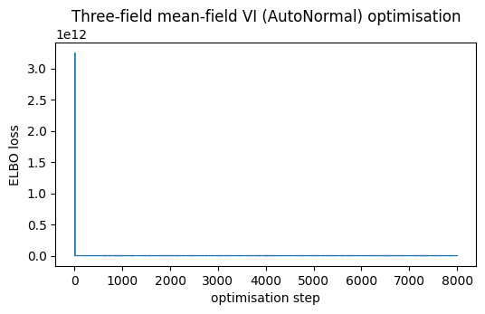
Mean-field VI fit in 13.3s · final ELBO loss 13978.3

Read off the three fields¶

lap = guide.sample_posterior(jr.PRNGKey(1), res.params, sample_shape=(600,))
pred = Predictive(model, posterior_samples=lap,
                  return_sites=["mu_field", "sigma_field", "xi_field", "f_xi_s",
                                "beta_ls", "cov_ls"])
draws = pred(jr.PRNGKey(2), Xn)

mu_field = np.asarray(draws["mu_field"])
sigma_field = np.asarray(draws["sigma_field"])
xi_field = np.asarray(draws["xi_field"])
f_xi = np.asarray(draws["f_xi_s"])
mu_med = mu_field.mean(0)
sig_med = sigma_field.mean(0)
xi_med = xi_field.mean(0)

print(f"μ(s) range : {mu_med.min():.1f} -> {mu_med.max():.1f} °C")
print(f"σ(s) range : {sig_med.min():.2f} -> {sig_med.max():.2f} °C")
print(f"ξ(s) range : {xi_med.min():+.3f} -> {xi_med.max():+.3f} "
      f"(global ξ in nb 07/08 was ≈ -0.19)")

beta = np.asarray(draws["beta_ls"])              # (n, n_cov)
print("log-σ covariate effects (per 1 SD, 95% CI):")
for j, labj in enumerate(COV_LABELS):
    lo, hi = np.quantile(beta[:, j], [0.025, 0.975])
    flag = "← excludes 0" if (lo > 0 or hi < 0) else ""
    print(f"  β[{labj:13s}] = {beta[:, j].mean():+.3f}  ({lo:+.2f}, {hi:+.2f})  {flag}")

μ(s) range : 21.1 -> 43.4 °C
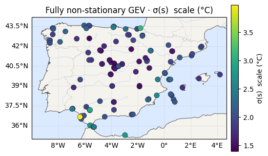
σ(s) range : 1.40 -> 3.98 °C
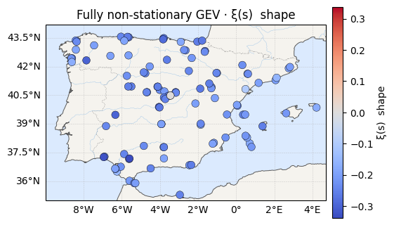
ξ(s) range : -0.338 -> +0.006 (global ξ in nb 07/08 was ≈ -0.19)
log-σ covariate effects (per 1 SD, 95% CI):
  β[elevation    ] = -0.093  (-0.11, -0.08)  ← excludes 0
  β[dist-to-coast] = -0.031  (-0.05, -0.01)  ← excludes 0

All three surfaces¶

Location, scale, and the newly-freed shape. Read the $\xi(s)$ panel sceptically — and against the per-station $\xi$ scatter of notebook 04.

xa = np.abs(xi_med).max()
for vals, label, cmap, clim in [
    (mu_med, "μ(s)  location (°C)", "RdYlBu_r", None),
    (sig_med, "σ(s)  scale (°C)", "viridis", None),
    (xi_med, "ξ(s)  shape", "coolwarm", (-xa, xa)),
]:
    ax = iberia_axes(figsize=(6.2, 5.2))
    sc = scatter_field(ax, lon, lat, vals, label=label, cmap=cmap)
    if clim is not None:
        sc.set_clim(*clim)
    ax.set_title(f"Fully non-stationary GEV · {label}")
    plt.show()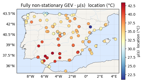

Did freeing ξ buy anything?¶

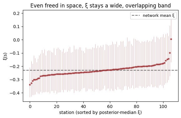
The decisive check is signal vs noise for the shape field, the same ratio as notebook 04: the spread of $\xi(s)$ across stations over the typical per-station 95% interval width. A value well below 1 means the across-station differences are small next to the uncertainty on each one — the map is mostly noise. (As in notebook 08 we fix the $f_\xi$ amplitude rather than learn it, so it is this ratio — not an imposed field amplitude — that carries the verdict.)

xi_lo = np.quantile(xi_field, 0.025, 0)
xi_hi = np.quantile(xi_field, 0.975, 0)
snr = xi_med.std() / (xi_hi - xi_lo).mean()
print(f"ξ(s) signal/noise = SD(median) / mean CI width = "
      f"{xi_med.std():.3f} / {(xi_hi - xi_lo).mean():.3f} = {snr:.2f}")
print(f"=> signal/noise {snr:.2f} << 1: the across-station spread of ξ(s) is small "
      "next to\n   the per-station uncertainty — little or no recoverable tail "
      "geography.")

fig, ax = plt.subplots(figsize=(6.4, 3.8))
order = np.argsort(xi_med)
x = np.arange(xi_med.size)
ax.errorbar(x, xi_med[order],
            yerr=[xi_med[order] - xi_lo[order], xi_hi[order] - xi_med[order]],
            fmt="o", ms=3, lw=0.5, color="#9b2226", ecolor="#bb5a5a", alpha=0.7)
ax.axhline(xi_med.mean(), ls="--", color="0.4", label="network mean ξ")
ax.set_xlabel("station (sorted by posterior-median ξ)")
ax.set_ylabel("ξ(s)")
ax.set_title("Even freed in space, ξ stays a wide, overlapping band")
ax.legend(fontsize=9)
plt.show()

ξ(s) signal/noise = SD(median) / mean CI width = 0.044 / 0.325 = 0.14
=> signal/noise 0.14 << 1: the across-station spread of ξ(s) is small next to
   the per-station uncertainty — little or no recoverable tail geography.

Return levels — does the map move?¶

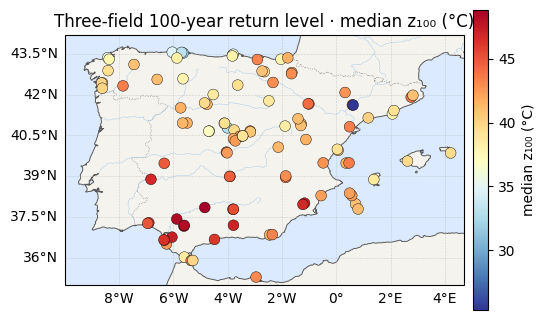
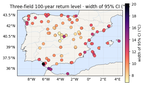
If the tail field is mostly noise, the $z_{100}$ map should look much like the two-field model’s, but with wider intervals — the extra freedom in $\xi$ adds variance without adding signal. That trade-off is the whole lesson.

RL = np.asarray(gev_return_level(
    100.0, jnp.asarray(mu_field), jnp.asarray(sigma_field),
    jnp.asarray(xi_field)))                    # (n, S)
rl_med = np.median(RL, 0)
rl_ciw = np.quantile(RL, 0.975, 0) - np.quantile(RL, 0.025, 0)
print(f"z100 median range : {rl_med.min():.1f} -> {rl_med.max():.1f} °C")
print(f"z100 95% CI width : {rl_ciw.mean():.1f} °C avg (max {rl_ciw.max():.1f}) "
      f"[nb 07 ≈ 2.7, nb 08 two-field for comparison]")

for vals, label, cmap in [(rl_med, "median z₁₀₀ (°C)", "RdYlBu_r"),
                          (rl_ciw, "width of 95% CI (°C)", "magma_r")]:
    ax = iberia_axes(figsize=(6.2, 5.2))
    scatter_field(ax, lon, lat, vals, label=label, cmap=cmap)
    ax.set_title(f"Three-field 100-year return level · {label}")
    plt.show()

z100 median range : 25.3 -> 48.8 °C
z100 95% CI width : 10.4 °C avg (max 20.1) [nb 07 ≈ 2.7, nb 08 two-field for comparison]

Takeaway — where non-stationarity stops paying¶

The machinery scales effortlessly: three independent GP fields fit in the same few seconds, and the location and scale surfaces match notebooks 07–08. But the shape tells the cautionary half of the story. Freed in space, $\xi(s)$ does not resolve into geography — its signal-to-noise stays well below one and its forest plot is the same wide, overlapping band we met at the very start in notebook 04. The data simply do not contain a recoverable map of the tail exponent; a spatial prior cannot conjure one, and paying for it in extra parameters only widens the return-level intervals.

That is the right note to end the build-up on. Spatial pooling is powerful exactly where there is structure to borrow — the location, and the scale (which, as the $\beta$ estimates above confirm, an elevation covariate carries better than a free GP) — and honest about where there is not. The useful working model for this dataset is notebook 08’s: a spatial location, an elevation-driven scale, and a global tail held in place by every station at once.