Arakawa C-Grid Masks

finitevolX provides three mask classes — Mask1D, Mask2D, Mask3D — that describe land/ocean geometry on an Arakawa C-grid. Every class operator in the package takes an optional mask class attribute of the matching dimension, so masks travel with operators rather than getting threaded through every call. See the Operator API section below for the full pattern and the stagger → mask field mapping.

The rest of this page documents Mask2D — the 2-D class — but the same factories (from_mask, from_dimensions, from_center, from_u_face …) and the same staggered-derivation pipeline are available on Mask1D (no v-face, no corner) and Mask3D (adds a w vertical face and native 3-D classification / stencil capability).

The Arakawa C-grid layout

Mask2D builds all staggered masks from a single cell-centre wet/dry field, following the Arakawa & Lamb (1977) grid layout:

y
^
:           :
w-----v-----w..
|           |
|           |
u     h     u
|           |
|           |
w-----v-----w..   > x

Point	Location	Variable
h	cell centre	tracers, height, pressure
u	east face	zonal velocity
v	north face	meridional velocity
xy_corner	NE corner (lenient)	vorticity
xy_corner_strict	NE corner (strict)	streamfunction

All staggered points use the same-index, positive half-step convention: u[j, i] is the east face of h[j, i], v[j, i] is the north face, and xy_corner[j, i] is the NE corner — matching CartesianGrid2D. See the Arakawa C-grid discretization notes for the underlying convention and a comparison with negative half-step alternatives.

Creating masks

All you need is a binary h-grid mask (True = ocean, False = land). The factory method derives everything else:

import numpy as np
from finitevolx import Mask2D

# Rectangular basin with land boundaries
n = 10
h_mask = np.ones((n, n), dtype=bool)
h_mask[0, :] = h_mask[-1, :] = False
h_mask[:, 0] = h_mask[:, -1] = False

# With an island
h_mask[4:7, 4:7] = False

masks = Mask2D.from_mask(h_mask)

For an all-ocean domain, use the shortcut:

masks = Mask2D.from_dimensions(ny=12, nx=12)

Or construct from any float field at a known grid position, where NaN marks dry cells:

# From a field at cell centres (T-points): SSH, temperature, pressure, …
masks = Mask2D.from_center(ssh_field)

# From a field at u-faces, v-faces, or xy-corners.  Pass `mode=` to
# choose the inversion strategy when the inverse mapping back to the
# h-grid is non-unique:
#   mode='permissive'  → h wet iff *any* surrounding face/corner wet
#   mode='conservative' → h wet iff *all* surrounding face/corner wet
masks = Mask2D.from_u_face(u_field, mode="permissive")
masks = Mask2D.from_v_face(v_field, mode="permissive")
masks = Mask2D.from_corner(vorticity_field, mode="conservative")

Staggered variable locations

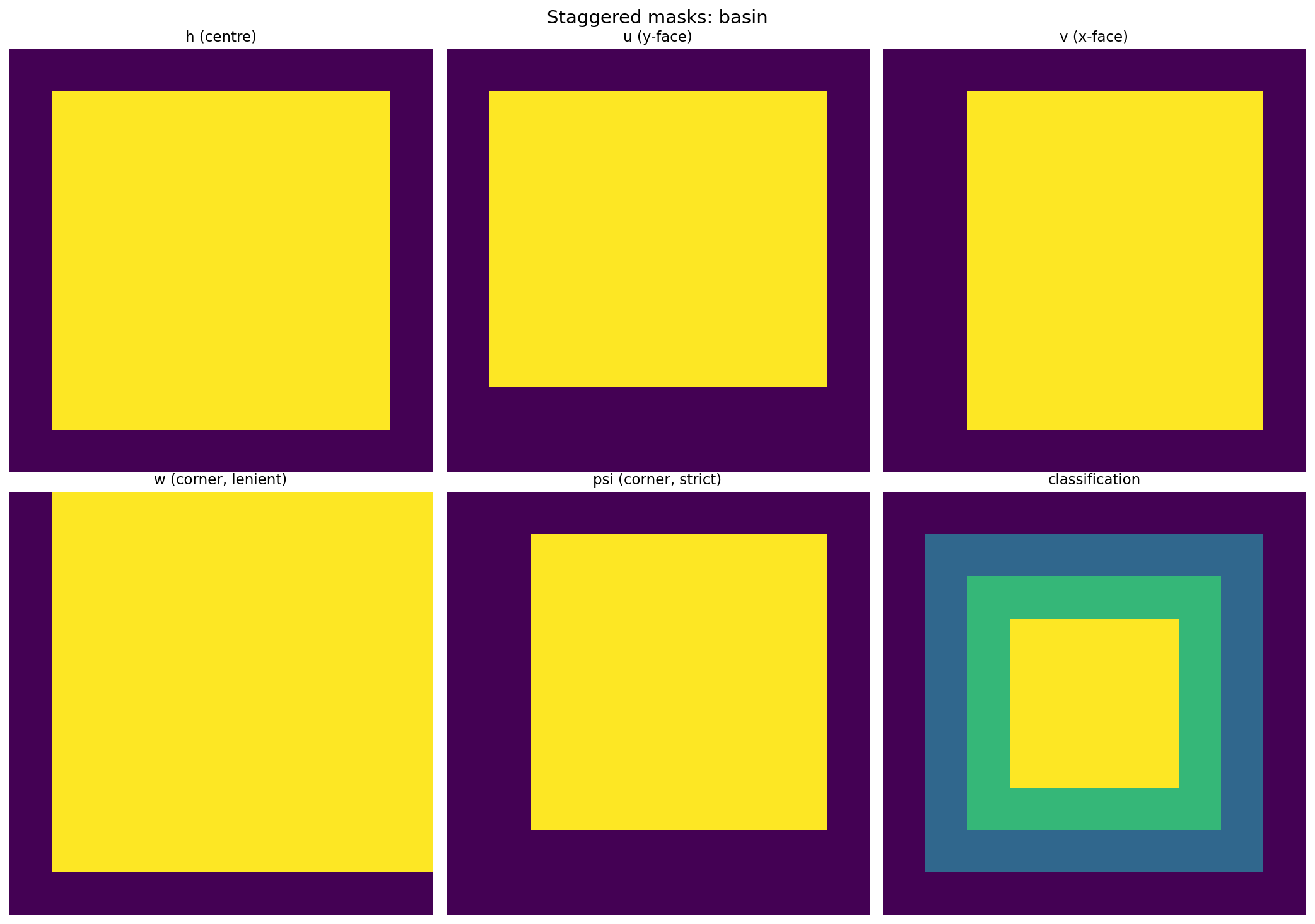
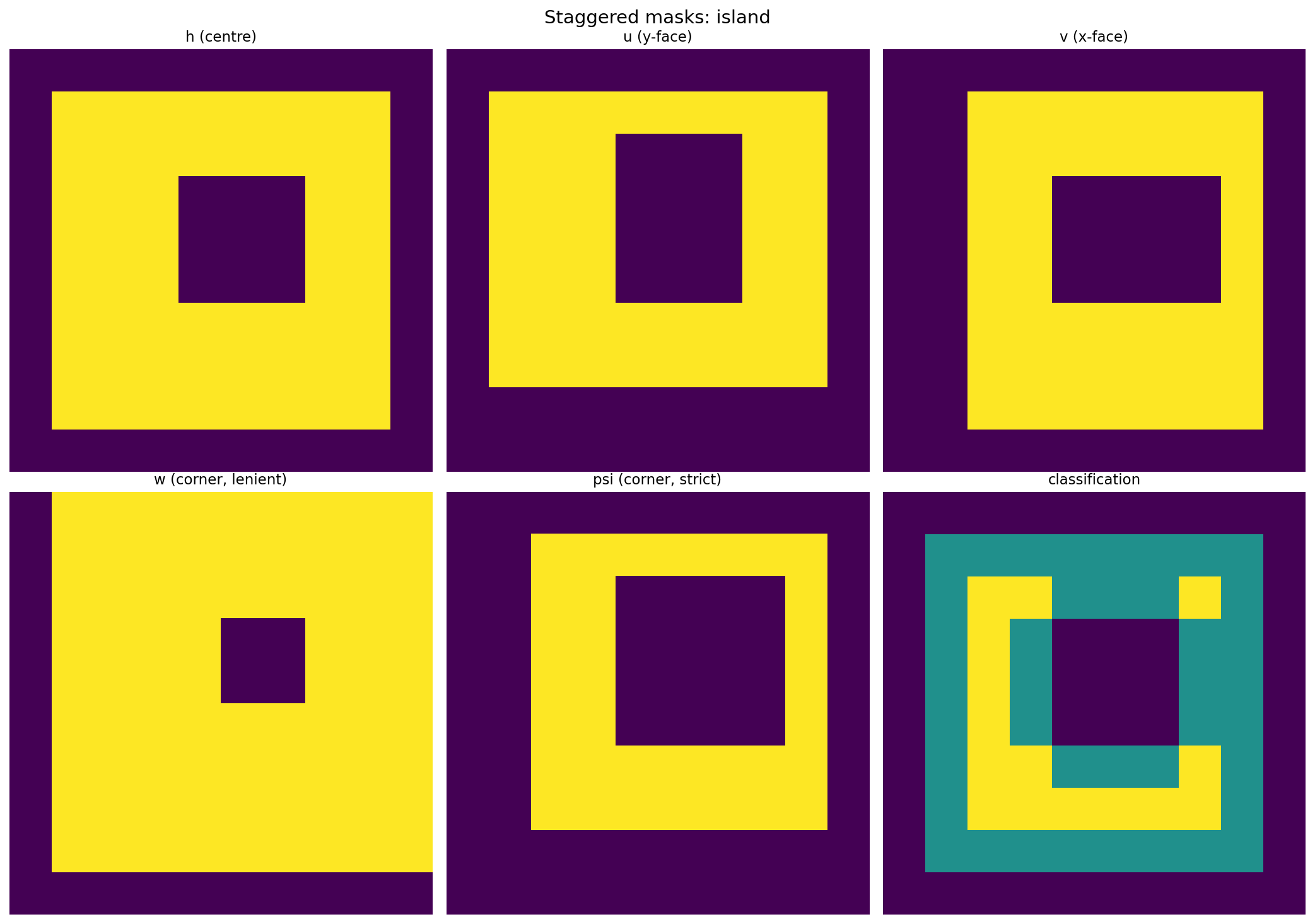
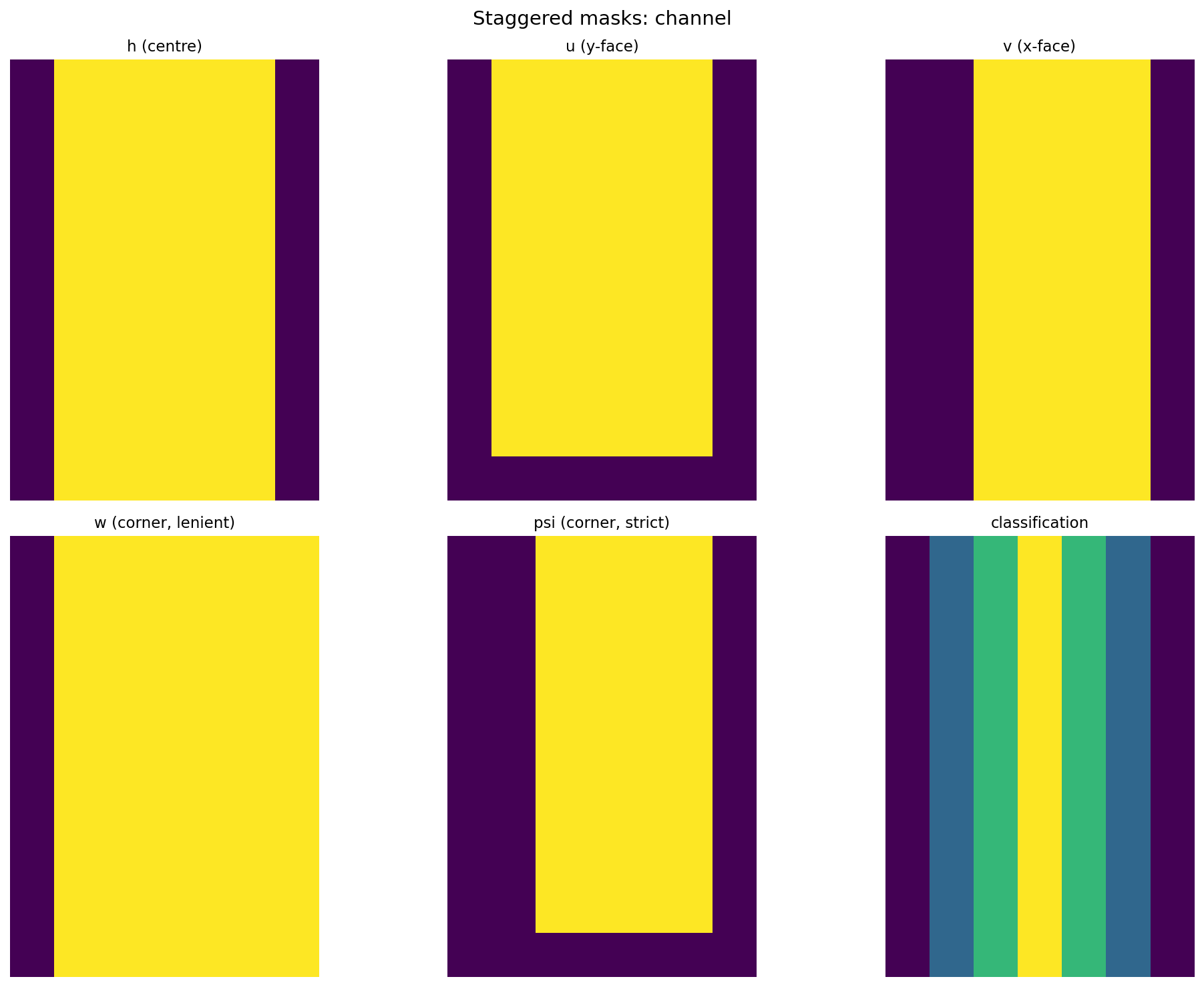
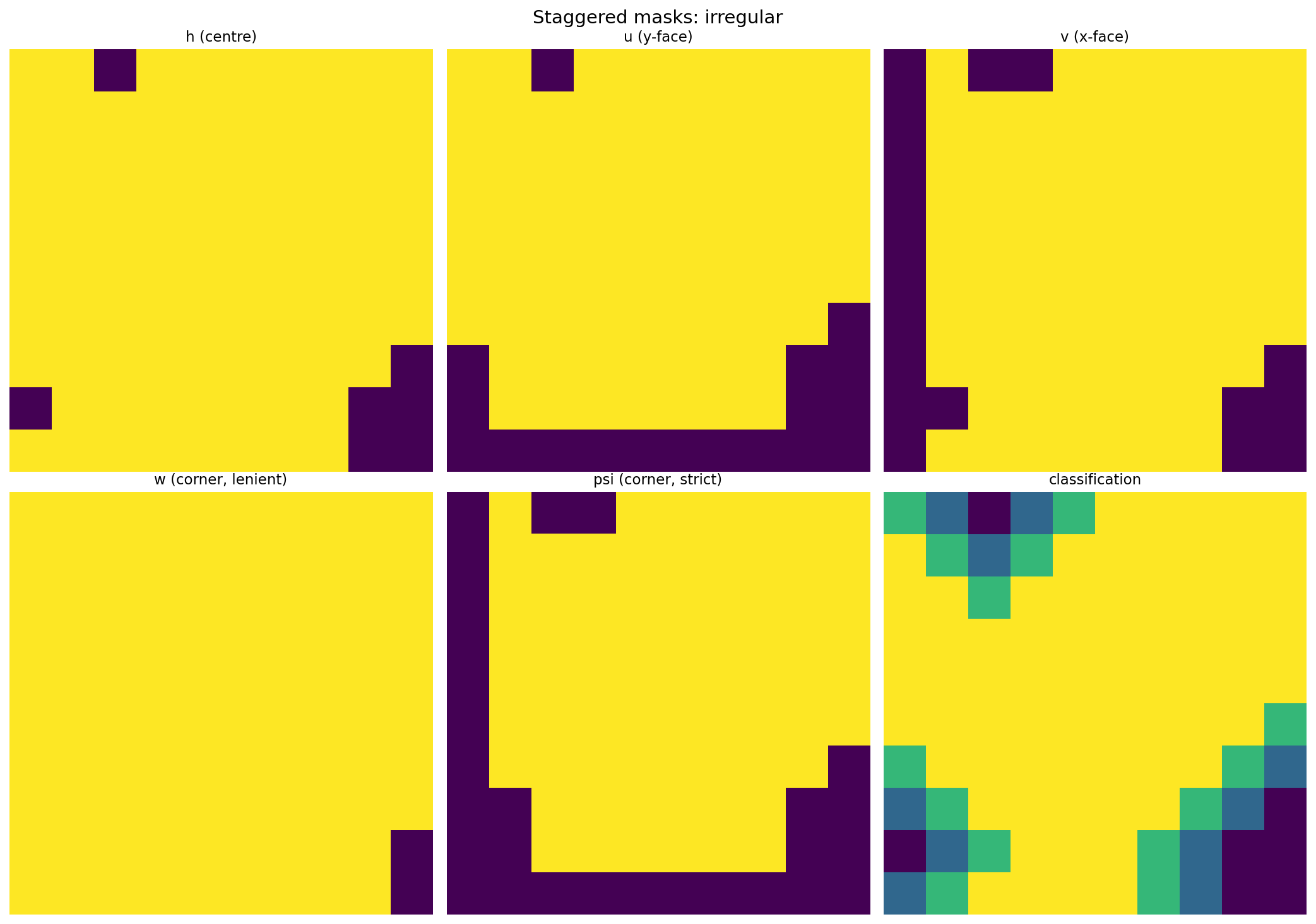
Each variable type sits at a different position within a grid cell. The figures below show the actual staggered positions for several domain topologies:

Rectangular basin

Basin with island

Zonal channel

Irregular coastline

Land / coast classification

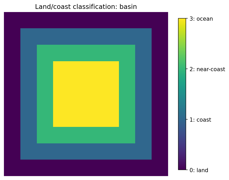
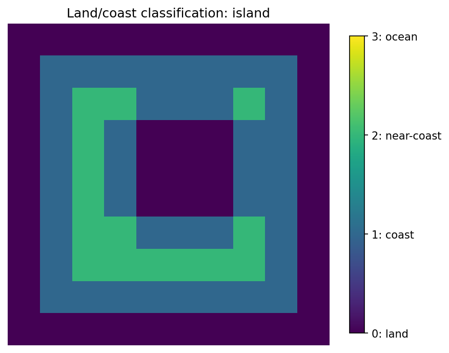
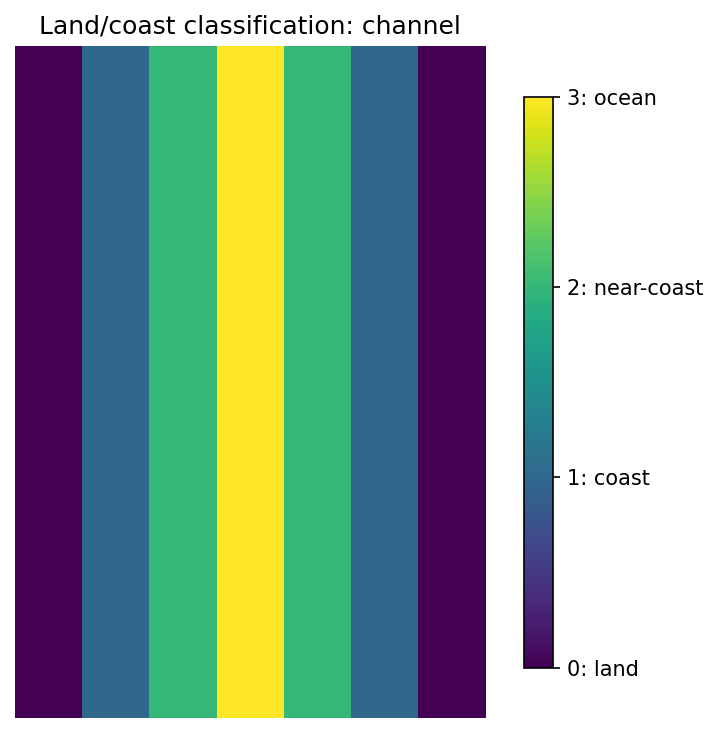
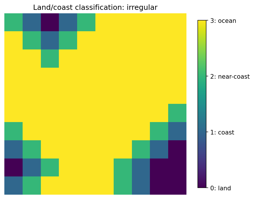
The mask includes a 4-level classification (0 = land, 1 = coast, 2 = near-coast, 3 = open ocean):

Rectangular basin

Basin with island

Zonal channel

Irregular coastline

Vorticity boundary classification

At xy-corner points, cells are classified based on their relationship to adjacent velocity faces:

• xy_corner_valid — interior: all 4 adjacent velocity faces are wet
• xy_corner_y_wall — on a vertical (y-direction) boundary
• xy_corner_x_wall — on a horizontal (x-direction) boundary
• xy_corner_convex — at convex corners (both boundary types)

Stencil capability and adaptive WENO

Each cell stores how many contiguous wet neighbours it has in each direction via StencilCapability2D. This drives adaptive stencil selection for WENO reconstruction near coastlines:

# Mutually-exclusive masks: largest usable stencil at each point
adaptive = masks.get_adaptive_masks(direction="x", source="h")
# adaptive[2]  → 1st-order upwind only
# adaptive[4]  → WENO3
# adaptive[6]  → WENO5
# adaptive[8]  → WENO7
# adaptive[10] → WENO9

Jupyter notebook

A complete interactive demo is available as a jupytext notebook: notebooks/demo_masks.py

---

Operator API: how operators consume masks

Every class operator in finitevolx takes an optional mask class attribute of the matching dimension. The mask travels with the operator; once constructed, method calls don't need to pass the mask through per call.

import finitevolx as fvx

grid = fvx.CartesianGrid2D.from_interior(64, 64, 1e6, 1e6)
mask = fvx.Mask2D.from_mask(h_mask)

# Mask as a class attribute — set once, consumed on every call.
diff = fvx.Difference2D(grid=grid, mask=mask)
adv  = fvx.Advection2D(grid=grid, mask=mask)
diff_op = fvx.Diffusion2D(grid=grid, mask=mask)

# Unmasked operators are the default — just omit `mask=`.
diff_noop = fvx.Difference2D(grid=grid)   # mask=None

The three-layer rule

finitevolx keeps masks out of the lowest two layers, so stencil and functional code stays coordinate-and-mask agnostic:

Layer	Example	Mask-aware?
Layer 1 — raw stencils	diff_x_fwd, avg_y_bwd, … in stencils.py	No
Layer 2 — functional helpers	_curl_2d, divergence_2d, diffusion_2d, kinetic_energy, enstrophy, geostrophic_velocity_sphere, arakawa_jacobian, …	No
Layer 3 — class operators	Difference2D, Interpolation2D, Divergence2D, Vorticity2D, Coriolis2D, Advection2D, Diffusion2D, MomentumAdvection2D, and their 1D / 3D / Spherical* siblings	Yes, via self.mask

If you call a Layer-2 functional helper and want masked output, apply the mask at the call site: ke = kinetic_energy(u, v) * mask.h.

Dimension → mask type mapping

Operators take the mask class matching their dimension:

Operator class	Mask type	Example
*1D (Difference1D, Interpolation1D, Advection1D)	Mask1D \| None	Difference1D(grid=g, mask=Mask1D.from_mask(h))
*2D (every 2-D operator)	Mask2D \| None	Advection2D(grid=g, mask=Mask2D.from_mask(h))
*3D (every 3-D operator)	Mask3D \| None	Diffusion3D(grid=g, mask=Mask3D.from_mask(h))

Spherical 2-D / 3-D operators take the Cartesian Mask2D / Mask3D — the mask geometry is coordinate-agnostic at the post-compute-multiply layer. A dedicated SphericalMask2D / SphericalMask3D is a TODO for future work.

Stagger → mask field mapping

The core convention is one operator output → one mask field, chosen by the operator's output stagger. Every operator follows the same mapping:

Output stagger	Mask field	Operators / methods
T (cell centre)	mask.h	divergence, laplacian, U→T / V→T / X→T differences and interpolations, Advection*, Diffusion*, BiharmonicDiffusion*
U (east face)	mask.u	T→U / X→U / V→U differences and interpolations, grad_perp u-component, Coriolis* du_cor, MomentumAdvection* du_adv
V (north face)	mask.v	T→V / X→V / U→V, grad_perp v-component, Coriolis* dv_cor, MomentumAdvection* dv_adv
X (NE corner)	mask.xy_corner_strict	curl, T→X / U→X / V→X, relative & potential vorticity, pv_flux_* U/V-stagger outputs where applicable

The X-output mapping uses the strict 4-of-4 corner mask (xy_corner_strict) because a corner-output value is trusted only when all four surrounding T-cells are wet. The lenient xy_corner mask is not currently consumed by any operator — it's available for users building their own.

Four patterns for mask application

Under the hood, operators apply masks in one of four patterns depending on what's safe. You don't need to know which is which for normal usage — the result is always "dry cells at the output stagger are exactly 0" — but the distinctions matter when customising or inheriting:

Pattern 1 — Post-compute multiply. Used by the majority of operators: Difference*, Interpolation*, Vorticity3D, Spherical*. Compute the output as if all-ocean, then multiply by the stagger-matched mask field at the end. Cheap and simple.

Pattern 2 — Pass-down into sub-operators. Used by composed operators with no tricky division — Divergence2D, Vorticity2D, MomentumAdvection2D. The outer class wires its mask into every internal sub-operator at __init__ time, so intermediate staggered fields are already zero at dry cells. The outer method trusts the pass-down and typically doesn't need an extra multiply.

• Special case for Vorticity2D.potential_vorticity: the (zeta + f) / h division would produce NaN at every dry X-corner under pass-down (because h_on_q == 0). The method preserves the existing "NaN at wet zero-thickness" sentinel but replaces mask-induced NaNs with exact 0 via a final jnp.where(mask.xy_corner_strict, out, 0). Same fix applies to SphericalVorticity2D.potential_vorticity.

Pattern 3 — Intermediate flux masking. Used by Diffusion2D and Diffusion3D only. Post-compute multiply is not sufficient for diffusion because the divergence at wet T-cells adjacent to land would be contaminated by polluted dry-side face fluxes. Instead the class wrappers apply the mask in three steps:

flux_x *= mask.u        # U-face stage
flux_y *= mask.v        # V-face stage
tendency *= mask.h      # final output

The shared kernel is _diffusion_2d_impl(h, kappa, dx, dy, mh, mu, mv) in finitevolx._src.diffusion.diffusion; Diffusion3D vmaps it per-z-slice with sliced masks (Pattern B in #209's terminology).

Pattern 4 — Final-only multiply with mask-free inner harmonic. Used by BiharmonicDiffusion2D and BiharmonicDiffusion3D. The biharmonic operator is two successive harmonic Laplacians; the mask is applied only to the final ∇⁴ tendency via * mask.h. Critically, the inner harmonic Diffusion is deliberately built with mask=None even when the outer biharmonic has a mask — masking the intermediate Laplacian would zero lap1 at dry cells, which acts as a forced Dirichlet-0 BC for the second harmonic pass and corrupts the ∇⁴ stencil at wet cells adjacent to land. The same applies to the 3-D class.

Pattern A vs Pattern B for 3-D operators

The 3-D wrappers that vmap an inner 2-D operator over z-levels (Vorticity3D, Coriolis3D, Spherical*3D, BiharmonicDiffusion3D, MomentumAdvection3D) use Pattern A (post-compute): the inner 2-D op is always constructed mask=None and the 3-D wrapper owns the mask, applying * self.mask.<stagger> after the vmap and zero_z_ghosts. This is cleaner than trying to thread per-z mask slices into the vmap'd 2-D op.

Diffusion3D is the exception and uses Pattern B (vmap with per-z sliced masks) because its intermediate flux masking makes Pattern A incorrect. See the Diffusion module docstring for the implementation.

Advection hierarchy pre-build

Advection1D / Advection2D / Advection3D are the special case where "mask as field" matters for performance, not just ergonomics. When constructed with a mask, __init__ pre-builds the (2, 4, 6) adaptive stencil hierarchy via mask.get_adaptive_masks(...) — once, up-front — and stores the result on the operator. Every subsequent call then uses the cached hierarchy, narrowed at dispatch time (by the narrow_mask_hierarchy helper) to the subset of tiers the chosen reconstruction method needs:

adv = fvx.Advection2D(grid=grid, mask=mask)  # builds (2,4,6) hierarchies

# First call uses the cached hierarchies; no get_adaptive_masks recomputation.
dh_dt = adv(h, u, v, method="weno5")

# A second method call on the same instance reuses the cache and
# narrows to (2, 4) on the fly for WENO3.
dh_dt = adv(h, u, v, method="weno3")

This is the main reason the Advection API moved from a per-call mask= kwarg to a class field: masks under JIT now compile once per Advection* instance instead of once per (instance, method) pair.

Changing the mask on an operator

equinox Modules are immutable — op.mask = new_mask will raise. To "change" a mask on an operator, use eqx.tree_at to produce a new operator instance with the field updated:

import equinox as eqx

# Start with one mask ...
adv_summer = fvx.Advection2D(grid=grid, mask=summer_mask)

# ... and produce a new instance with a different mask.  The grid and
# reconstruction module are shared (no copy); only `mask` (and, for
# Advection, the pre-built hierarchies — eqx.tree_at reconstructs the
# __init__ path correctly for all affected fields) is swapped.
adv_winter = eqx.tree_at(lambda o: o.mask, adv_summer, winter_mask)

For composed operators (Divergence2D, Vorticity2D, MomentumAdvection2D, etc.) the outer self.mask is independent of the mask stored on the internal sub-operators, so you may also need to swap those — the simpler alternative is usually to just construct a fresh operator from scratch:

# Cleaner for composed ops
vort_winter = fvx.Vorticity2D(grid=grid, mask=winter_mask)

Migration from the old per-call kwarg API

Some operators used to take mask= as a per-call keyword argument. In the current API, the mask is always a class field. Translation:

# Old (removed)
adv = fvx.Advection2D(grid=grid)
adv(h, u, v, method="weno5", mask=mask)

cor = fvx.Coriolis2D(grid=grid)
cor(u, v, f, mask=mask)

# New
adv = fvx.Advection2D(grid=grid, mask=mask)
adv(h, u, v, method="weno5")

cor = fvx.Coriolis2D(grid=grid, mask=mask)
cor(u, v, f)

Diffusion2D, Diffusion3D, diffusion_2d, Difference2D.grad_perp, kinetic_energy, enstrophy, and potential_enstrophy used to take raw-array mask_h / mask_u / mask_v keyword arguments. Those are all removed:

• Diffusion2D / Diffusion3D take a Mask2D / Mask3D class field instead.
• diffusion_2d (the Layer-2 free function) is mask-free. If you want masked diffusion, use the class operator.
• Difference2D.grad_perp uses the self.mask class field (set on Difference2D at construction).
• kinetic_energy / enstrophy / potential_enstrophy are Layer-2 mask-free. Apply masks at the call site:

ke = fvx.kinetic_energy(u, v) * mask.h
z  = fvx.enstrophy(omega)     * mask.xy_corner_strict
pe = fvx.potential_enstrophy(q, h) * mask.xy_corner_strict