Forward simulation of a steady-state Gaussian plume
This notebook exercises the forward model in plumax.gauss_plume: a steady-state Gaussian plume with Briggs-McElroy-Pooler dispersion coefficients, ground reflection, and wind-frame rotation. We’ll render a few diagnostic views (horizontal column, vertical centerline slice, crosswind Gaussian profile), sweep over the six Pasquill-Gifford stability classes to see how dispersion scales, and finish by running the NumPyro model in prior-predictive mode to visualise the range of plumes implied by our emission-rate prior.
The fit-and-infer companion notebooks (02, 03) pick up from here: 02_emission_rate_parameter_estimation inverts a downwind transect to recover Q, and 03_plume_state_estimation treats Q as a time-varying latent state recovered from a sequence of observations.
import warnings


warnings.filterwarnings("ignore", message=r".*IProgress.*")

import jax
import jax.numpy as jnp
import matplotlib.pyplot as plt
import numpy as np
import numpyro
from numpyro.infer import Predictive

from plumax.gauss_plume import (
    BRIGGS_DISPERSION_PARAMS,
    STABILITY_CLASSES,
    gaussian_plume_model,
    plume_concentration,
    simulate_plume,
)


numpyro.set_host_device_count(1)
rng = np.random.default_rng(0)
1. Run a single forward simulation
Set up a canonical scenario: a ground-level leak of 0.1 kg/s from a 2 m stack, with a 5 m/s westerly wind (meteorological convention: wind_direction = 270° means wind from the west). Neutral stability (class D) is a good default for a daylight scenario with moderate wind.
ds = simulate_plume(
    emission_rate=0.1,
    source_location=(0.0, 0.0, 2.0),
    wind_speed=5.0,
    wind_direction=270.0,  # wind FROM the west
    stability_class="D",
    domain_x=(-50.0, 1200.0, 251),
    domain_y=(-180.0, 180.0, 181),
    domain_z=(0.0, 80.0, 21),
    background_conc=0.0,
)

print(ds)
print(f"\nPeak concentration:        {float(ds['concentration'].max()):.3e} kg/m^3")
print(
    f"Peak column concentration: {float(ds['column_concentration'].max()):.3e} kg/m^2"
)
<xarray.Dataset> Size: 4MB
Dimensions: (x: 251, y: 181, z: 21)
Coordinates:
* x (x) float64 2kB -50.0 -45.0 ... 1.195e+03 1.2e+03
* y (y) float64 1kB -180.0 -178.0 -176.0 ... 178.0 180.0
* z (z) float64 168B 0.0 4.0 8.0 12.0 ... 72.0 76.0 80.0
Data variables:
concentration (x, y, z) float32 4MB 0.0 0.0 ... 4.797e-08 4.055e-08
column_concentration (x, y) float64 363kB 0.0 0.0 ... 1.201e-05 1.15e-05
Attributes: (12/14)
title: Steady-state Gaussian plume (JAX)
emission_rate: 0.1
emission_rate_units: kg/s
source_x: 0.0
source_y: 0.0
source_z: 2.0
... ...
wind_direction: 270.0
wind_direction_units: degrees from North (meteorological)
wind_u: 5.0
wind_v: 9.184850993605148e-16
stability_class: D
background_concentration: 0.0
Peak concentration: 8.606e-04 kg/m^3
Peak column concentration: 3.444e-03 kg/m^2
2. Horizontal column view
Summing the concentration along z gives the column density the satellite would retrieve. The plume is a characteristic fan: narrow near the source, broadening with downwind distance as σ_y(x) grows.
fig, ax = plt.subplots(figsize=(10, 4.5))
im = ax.pcolormesh(
    ds["x"].values,
    ds["y"].values,
    ds["column_concentration"].T.values,
    cmap="inferno",
    shading="auto",
)
plt.colorbar(im, ax=ax, label="column concentration [kg/m²]")
ax.scatter(
    [0.0],
    [0.0],
    marker="*",
    s=220,
    color="white",
    edgecolor="black",
    linewidth=1.2,
    zorder=5,
    label="source",
)
ax.set_xlabel("x  [m]  (downwind →)")
ax.set_ylabel("y  [m]  (crosswind)")
ax.set_title(
    "Gaussian plume — horizontal column view (class D, Q = 0.1 kg/s, U = 5 m/s)"
)
ax.legend(loc="upper right")
plt.tight_layout()
plt.show()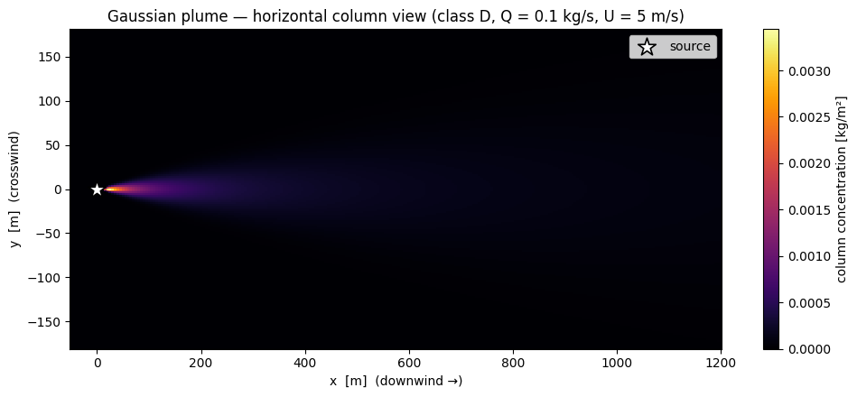
3. Vertical centerline slice and crosswind profile
A vertical slice along the plume centerline (y = 0) shows the ground-reflected vertical Gaussian — the concentration spreads upward from the stack and is reflected at z = 0, keeping all the mass in the boundary layer. The crosswind profile at a downwind distance of 500 m is a Gaussian in y, whose width is σ_y(500 m).
fig, (ax1, ax2) = plt.subplots(1, 2, figsize=(12, 4.3))

# Vertical centerline slice.
centerline = ds["concentration"].sel(y=0.0, method="nearest").T
im1 = ax1.pcolormesh(
    ds["x"].values,
    ds["z"].values,
    centerline.values,
    cmap="viridis",
    shading="auto",
)
plt.colorbar(im1, ax=ax1, label="concentration [kg/m³]")
ax1.scatter(
    [0.0],
    [2.0],
    marker="*",
    s=160,
    color="white",
    edgecolor="black",
    linewidth=1.0,
    zorder=5,
)
ax1.set_xlabel("x  [m]")
ax1.set_ylabel("z  [m]")
ax1.set_title("Vertical slice along y = 0")

# Crosswind Gaussian profile at x = 500 m, z = 2 m.
cross = ds["concentration"].sel(x=500.0, z=2.0, method="nearest").values
ax2.plot(ds["y"].values, cross, color="#c0392b", linewidth=2.0)
ax2.set_xlabel("y  [m]  (crosswind)")
ax2.set_ylabel("concentration [kg/m³]")
ax2.set_title("Crosswind profile at x = 500 m, z = 2 m")
ax2.grid(alpha=0.3)

plt.tight_layout()
plt.show()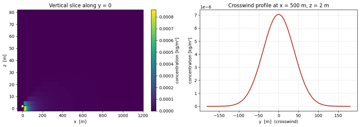
4. Stability-class sweep
The six Pasquill-Gifford classes span from A (very unstable, strong daytime convection) to F (very stable, clear calm nights). Unstable classes disperse pollutants aggressively, spreading the plume quickly and lowering peak concentration; stable classes produce long, thin plumes with high peak near the source. Below we plot the centerline (y = 0, z = 0) concentration as a function of downwind distance for all six classes.
x_line = jnp.linspace(20.0, 2500.0, 400)
y_line = jnp.zeros_like(x_line)
z_line = jnp.zeros_like(x_line)

fig, ax = plt.subplots(figsize=(10, 4.5))
colors = plt.cm.viridis(np.linspace(0.0, 1.0, len(STABILITY_CLASSES)))
for stab, color in zip(STABILITY_CLASSES, colors, strict=True):
    conc = plume_concentration(
        x_line,
        y_line,
        z_line,
        0.0,
        0.0,
        2.0,  # source
        5.0,
        0.0,  # wind components (westerly at 5 m/s)
        0.1,  # emission rate
        BRIGGS_DISPERSION_PARAMS[stab],
    )
    ax.plot(
        np.asarray(x_line),
        np.asarray(conc),
        label=f"class {stab}",
        color=color,
        linewidth=1.8,
    )

ax.set_xlabel("downwind distance  [m]")
ax.set_ylabel("ground-level concentration [kg/m³]")
ax.set_yscale("log")
ax.set_title("Centerline concentration vs downwind distance, by stability class")
ax.grid(alpha=0.3, which="both")
ax.legend(ncols=2, loc="upper right")
plt.tight_layout()
plt.show()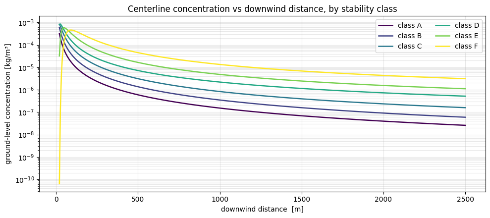
5. Prior-predictive check with NumPyro
The gaussian_plume_model defined in plumax.gauss_plume.inference wraps the forward model with a LogNormal emission-rate prior and a HalfNormal background prior. Running the model forward with observations=None samples predicted concentrations for each prior draw; this is a prior-predictive check, a useful sanity test that our priors are neither far too loose nor too tight for the scenario.
x_obs_np = np.linspace(200.0, 2000.0, 19)
y_obs_np = np.zeros_like(x_obs_np)
z_obs_np = np.ones_like(x_obs_np)

receptor_coords = (jnp.asarray(x_obs_np), jnp.asarray(y_obs_np), jnp.asarray(z_obs_np))

predictive = Predictive(gaussian_plume_model, num_samples=200)
samples = predictive(
    jax.random.PRNGKey(0),
    observations=None,
    receptor_coords=receptor_coords,
    source_location=(0.0, 0.0, 2.0),
    wind_u=5.0,
    wind_v=0.0,
    stability_class="D",
    prior_emission_rate_mean=0.1,
    prior_emission_rate_std=0.05,
    infer_stability=False,
)

prior_Q = np.asarray(samples["emission_rate"])
prior_obs = np.asarray(samples["obs"])  # shape (200, 19)
Below we plot:
The marginal prior over the emission rate Q (LogNormal centred on 0.1 kg/s).
The induced prior over ground-level concentrations along the transect, shown as the 5–95 % envelope and the median.
fig, (ax1, ax2) = plt.subplots(1, 2, figsize=(12, 4.3))

ax1.hist(prior_Q, bins=40, color="#2c3e50", alpha=0.85)
ax1.axvline(0.1, color="#c0392b", linestyle="--", linewidth=1.8, label="prior mean")
ax1.set_xlabel("emission rate Q  [kg/s]")
ax1.set_ylabel("count")
ax1.set_title("Prior samples — emission rate (LogNormal)")
ax1.legend()

p05 = np.percentile(prior_obs, 5, axis=0)
p50 = np.percentile(prior_obs, 50, axis=0)
p95 = np.percentile(prior_obs, 95, axis=0)
ax2.fill_between(x_obs_np, p05, p95, alpha=0.3, color="#2c3e50", label="prior 5–95 %")
ax2.plot(x_obs_np, p50, color="#2c3e50", linewidth=2.0, label="prior median")
ax2.set_xlabel("downwind distance  [m]")
ax2.set_ylabel("predicted concentration [kg/m³]")
ax2.set_title("Prior-predictive concentration along transect")
ax2.grid(alpha=0.3)
ax2.legend()

plt.tight_layout()
plt.show()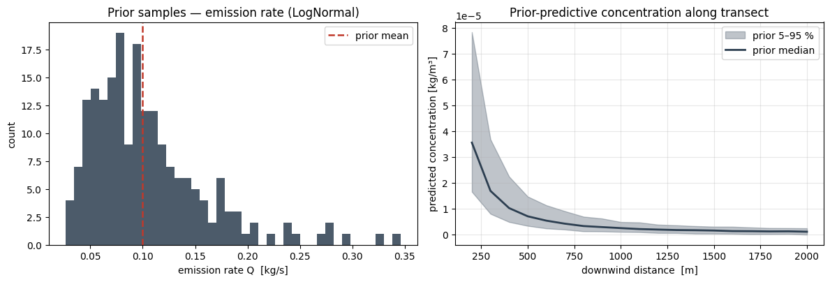
Summary
We have a fully differentiable, JIT-compiled forward model for a steady-state Gaussian plume, wrapped as an xarray.Dataset for diagnostic plotting and as a NumPyro-compatible function for Bayesian workflows. In the next notebook we invert this model — given a set of downwind concentrations, recover the emission rate Q. The one after that treats Q as a time-varying state in a random-walk state-space model.