Part I — The real problem and the real data

Before any mathematics: what is physically out there, what the instruments return, and the one running example carried through every later page.

I.1 The task, in three phases¶

Phase	Question	What is random
A — Discovery	Where are the sources we don’t yet know about?	Locations
B — Monitoring	For sources we know, when are they emitting?	State over time
C — Estimation	How much does each emit, and what is the total?	Rates and their sum

The three phases need different mathematical objects because a different thing is uncertain in each. Part II builds those objects; Part III maps them back onto the phases.

I.2 What is actually out there¶

Methane sources in an oil-and-gas basin come in two physical kinds, and the distinction is one of scale:

Point sources

A single failed valve, an unlit flare, a tank vent. Spatial extent of metres; a compact, high-contrast plume. Rates from tens of $\mathrm{kg\,h^{-1}}$ to several $\mathrm{t\,h^{-1}}$ . Often intermittent: on for hours, off for days.

Area (diffuse) sources

Thousands of small leaks across an old field, a landfill face, a wetland. Extent of kilometres; a broad, low-contrast enhancement. Individually tiny, collectively large. Usually persistent.

Two empirical facts drive everything downstream:

Rates are heavy-tailed. A few percent of point sources (“super-emitters”) carry a large share of the total.
Whether something is a point or an area source depends on what you look with. A cluster of twenty small pads inside one coarse pixel is, to that instrument, an area source. To a fine imager it is twenty points.

I.3 What the instruments give¶

Every instrument is characterised by four numbers.^[1]

Quantity	Symbol	Coarse mapper	Fine imager	Units
pixel size	$\Delta x$	$\approx 5$ –7	$\approx 0.03$	km
revisit	$\Delta t$	$\approx 1$	$\approx 5$ (or tasked)	d
per-source detection limit	$s_{\min}$	$\approx$ several $\times 10^3$	$\approx 10^2$ –10³	$\mathrm{kg\,h^{-1}}$
per-pixel precision	$\sigma_r$	$\approx 10$	$\approx 100+$	ppb

Consequences:

Coarse mapper

Fine imager

Sees almost every point source in the §I.2 example only as part of a pixel aggregate. It sees area sources well, after averaging many days.

I.4 Data products¶

Product	What it is	Units
L2 $\mathrm{XCH_4}$	column-mean mole fraction per pixel	ppb
enhancement $f(x)$	$\mathrm{XCH_4}$ minus local background	ppb
plume mask	pixels flagged as plume	—
rate estimate	per-plume flux from mask + wind (e.g. IME method)	$\mathrm{kg\,h^{-1}}$
wind $\mathbf{U}$	10 m wind vector from reanalysis	$\mathrm{m\,s^{-1}}$
bottom-up inventory	gridded prior emission density	$\mathrm{kg\,h^{-1}\,km^{-2}}$
infrastructure database	candidate site coordinates $c_j$ (pads, compressors)	km, km

I.5 The running example¶

A $40\,\mathrm{km} \times 40\,\mathrm{km}$ study region $S$ in the Permian Basin, partitioned into four $20\,\mathrm{km} \times 20\,\mathrm{km}$ cells $A_1,\dots,A_4$ .

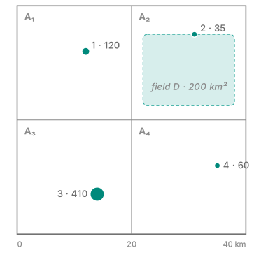
Map of the 40 km by 40 km study region with four cells, four point sources and one diffuse field — Figure 1:The study region $S$ . Dots are the point sources, sized by on-state rate ( $\mathrm{kg\,h^{-1}}$ ); the dashed patch is the diffuse old field $D$ inside $A_2$ .

Point sources (true, unknown to us at the start):

$k$	$x_k$ (km)	$s_k$ on ( $\mathrm{kg\,h^{-1}}$ )	$\pi_k$	in
1	(12, 32)	120	0.9	$A_1$
2	(31, 35)	35	1.0	$A_2$
3	(14, 7)	410	0.3	$A_3$
4	(35, 12)	60	1.0	$A_4$

$\pi_k$ is the fraction of time source $k$ is on. Source 3 is a large intermittent emitter: a blowdown that fires roughly one day in three.

Area source: an old field $D \subset A_2$ of $200\,\mathrm{km^2}$ with flux density $e(x) \approx 2\ \mathrm{kg\,h^{-1}\,km^{-2}}$ , giving $400\ \mathrm{kg\,h^{-1}}$ diffuse.

True totals:

Time-averaged (what an inventory wants)

Instantaneous (all sources on)

\begin{aligned} \text{point, time-averaged } (\pi_k s_k): &\quad 108 + 35 + 123 + 60 = 326\ \mathrm{kg\,h^{-1}}\\ \text{diffuse:} &\quad 400\ \mathrm{kg\,h^{-1}}\\ \text{basin, time-averaged:} &\quad 726\ \mathrm{kg\,h^{-1}} \end{aligned}

(1)

Instruments:

	$\Delta x$	revisit	$s_{\min}$	What it sees here
Coarse mapper	$\approx 7$ km	daily	$\approx 5000\ \mathrm{kg\,h^{-1}}$	no single point source
Fine imager	$\approx 0.03$ km	every 5 d	$\approx 100\ \mathrm{kg\,h^{-1}}$	sources 1 and 3, when they are on and the scene is clear

I.6 Notation and units¶

Fixed for the whole section.

Full symbol table (click to expand)

Symbol	Meaning	Units
$S$	spatial domain	—
$x \in S$	location (easting, northing)	km, km
$T = [0, T_{\mathrm{end}}]$	time window	d
$t \in T$	a time	d
$X$	generic index set: $S$ , $T$ , or $S \times T$	—
$A \subset X$	a region or interval	—
$\lvert A \rvert$	area (or length) of $A$	$\mathrm{km^2}$ (d)
$\delta_x$	point mass at $x$	—
$N(A)$	number of point sources in $A$	—
$\lambda(A)$ , $\lambda(x)$	expected count in $A$ ; source density	—, $\mathrm{km^{-2}}$
$\lambda(t)$	event rate	$\mathrm{d^{-1}}$
$s_k$	on-state rate of point source $k$	$\mathrm{kg\,h^{-1}}$
$s_0$	reference rate, $1\ \mathrm{kg\,h^{-1}}$	$\mathrm{kg\,h^{-1}}$
$\pi_k$	persistence (fraction of time on) of source $k$	—
$G(\mathrm{d}\pi \mid u)$	distribution of persistence given on-state rate	—
$p_{\mathrm{camp}}$	probability a source is detected at least once over a campaign	—
$\lambda_{\ge}$ , $R$	count intensity of sources above the floor $u_{\mathrm{floor}}$ ; $R = \rho([u_{\mathrm{floor}},\infty))$	$\mathrm{km^{-2}}$ , —
$e(x)$	diffuse flux density	$\mathrm{kg\,h^{-1}\,km^{-2}}$
$\mu(A)$	total emission rate from $A$ (point + diffuse)	$\mathrm{kg\,h^{-1}}$
$\mu_{\mathrm{pt}}$ , $\mu_{\mathrm{df}}$	atomic and diffuse parts of $\mu$	$\mathrm{kg\,h^{-1}}$
$H(A)$	prior expected emission from $A$	$\mathrm{kg\,h^{-1}}$
$u_k$	dimensionless rate $s_k/s_0$	—
$\rho(\mathrm{d}u)$	Lévy measure over dimensionless rates $u$	—
$G(A)$	fraction of basin total from $A$	—
$f(x)$	$\mathrm{XCH_4}$ enhancement	ppb
$m(x)$ , $k(x,x')$	mean, covariance kernel of a field	ppb, $\mathrm{ppb^2}$
$g(x)$	log source density, $\log\lambda(x)$	—
$\Delta x$ , $\Delta t$	pixel size, revisit interval	km, d
$C_\Delta$	coarsening operator: $\mu \mapsto$ pixel totals	—
$\mathcal{T}$	atmospheric transport operator: $\mu \mapsto f$	ppb per $\mathrm{kg\,h^{-1}}$
$\mathbf{U}$ , $U$	10 m wind vector (east, north); its speed $U = \lVert\mathbf{U}\rVert$	$\mathrm{m\,s^{-1}}$
$p(x,s)$	detection probability	—
$s_{\min}$	detection limit	$\mathrm{kg\,h^{-1}}$
$c_j$ , $Z_j$	candidate site $j$ ; its emitting indicator	km km, —
$m_k$ , $M(t)$	event mass; cumulative mass by $t$	kg
$\lambda^*(t)$ , $\mathcal{H}_t$	conditional intensity; history before $t$	$\mathrm{d^{-1}}$ , —

Footnotes¶

Values are indicative orders of magnitude; check current mission specifications before relying on them.
↩