Band-integrated forward model + plume injection

Band integration, forward models & nB-LUT plume injection¶

The line-by-line LUT from notebook 01 gives $\sigma(\nu, T, P)$ at fine wavenumber resolution. Real multispectral instruments observe band-integrated radiance — each band $b$ collects photons across a wavelength window weighted by its Spectral Response Function (SRF) $f_b(\lambda)$ . This notebook closes the loop from the HR LUT to per-pixel band radiance via three steps:

Forward models side-by-side. Three flavours of Beer–Lambert — exact, Maclaurin, and Taylor — exposed through plumax.radtran.forward. We plot them at a single wavenumber to see where the linearisations break.
SRF band integration. Build a Gaussian SRF at two S2-like bands (B11 @ 1610 nm, B12 @ 2190 nm) and apply it to a per-wavelength transmittance spectrum.
Normalised-brightness LUT. Pre-tabulate $nB_b(\Delta X) = \int f_b(\lambda)\, \exp[-\mathrm{AMF}\cdot\sigma(\lambda)\cdot\Delta X]\,d\lambda\,/\,\int f_b(\lambda)\,d\lambda$ over a 1-D grid of column enhancements, then apply it per-pixel to a clean synthetic scene via inject_plume.

Notebook 05 builds on this to do a matched-filter retrieval. The physics is derived in 00_hapi_lut_derivation.md (same Beer–Lambert start) and motivated by Orbio’s Project Eucalyptus Radiative_Transfer.md — which argues that at the single-slab, band-integrated level the nB-LUT cancels most of the aerosol / albedo ignorance to first order.

import warnings
from pathlib import Path


warnings.filterwarnings("ignore")

import matplotlib.pyplot as plt
import numpy as np
import xarray as xr

from plumax.gauss_plume import simulate_plume
from plumax.radtran import (
    InstrumentSpec,
    ObservationGeometry,
    build_nb_lut,
    forward_maclaurin_normalized,
    forward_nonlinear_normalized,
    inject_plume,
    lookup_nb,
)


# Built by 01_hapi_lut_ch4.ipynb into a per-user cache, outside the repository.
LUT_PATH = Path.home() / ".cache" / "plumax" / "hapi_lut" / "ch4_absorption_lut.nc"
assert LUT_PATH.exists(), f"Run 01_hapi_lut_ch4.ipynb first — missing {LUT_PATH}"

ch4_lut = xr.open_dataset(LUT_PATH)
nu_grid = ch4_lut["wavenumber"].values
wl_grid = ch4_lut["wavelength"].values
print(
    f"LUT spans {nu_grid.min():.0f}-{nu_grid.max():.0f} cm^-1 "
    f"(λ ≈ {wl_grid.max():.0f}-{wl_grid.min():.0f} nm), {nu_grid.size} points."
)

LUT spans 4000-4500 cm^-1 (λ ≈ 2500-2222 nm), 10000 points.

1. Atmospheric state and viewing geometry¶

Mid-troposphere state — same as notebook 03. The ObservationGeometry dataclass packs the solar / viewing angles plus the single-slab vertical path into one immutable object; the air-mass factor is derived from the plane-parallel formula.

geom = ObservationGeometry(
    sza_deg=30.0,
    vza_deg=0.0,  # nadir
    path_length_cm=8e5,  # 8 km tropospheric column
)
T_K = 260.0
p_atm = 0.6
print(f"AMF = {geom.air_mass_factor:.3f}")

# Background CH4 mixing ratio (current global mean ~1.9 ppm).
VMR_BG = 1.9e-6

AMF = 2.155

2. Forward-model flavours¶

All three models return a ForwardResult(radiance, jacobian, transmittance). Below we sweep $\Delta\mathrm{VMR}$ at the strongest CH $_4$ absorption line in our LUT (~4300 cm⁻¹, ≈ 2326 nm) and plot the normalised radiance $L_\text{norm} = L/L_\text{bg}$ . The Maclaurin-1 variant is the linear matched-filter assumption; the Taylor-1 around the background collapses to the same at first order (we show only Maclaurin here). The nonlinear curve exposes where linearisations break.

# Use a representative absorption line — the median of the nonzero σ values
# in the Q-branch. The LUT's absolute peak is unusually strong and would push
# the Maclaurin expansions off-scale before they can trace the nonlinear curve.
sigma_at_T_p = (
    ch4_lut["absorption_cross_section"].interp(temperature=T_K, pressure=p_atm).values
)
strong_mask = sigma_at_T_p > np.quantile(sigma_at_T_p, 0.95)
nu_strong = float(nu_grid[np.where(strong_mask)[0][len(np.where(strong_mask)[0]) // 2]])
sigma_strong = float(sigma_at_T_p[np.argmin(np.abs(nu_grid - nu_strong))])
print(
    f"Representative line: ν = {nu_strong:.1f} cm^-1 (λ = {1e7 / nu_strong:.1f} nm), "
    f"σ = {sigma_strong:.2e} cm²/molec"
)

delta_vmrs = np.linspace(0, 0.6e-6, 61)  # 0 to 0.6 ppm — the matched-filter regime
L_nl = np.empty_like(delta_vmrs)
L_m1 = np.empty_like(delta_vmrs)
L_m2 = np.empty_like(delta_vmrs)

common_kw = dict(
    T_K=T_K,
    p_atm=p_atm,
    path_length_cm=geom.path_length_cm,
    amf=geom.air_mass_factor,
)
for i, dvmr in enumerate(delta_vmrs):
    L_nl[i] = forward_nonlinear_normalized(
        ch4_lut,
        np.array([nu_strong]),
        vmr_background=VMR_BG,
        delta_vmr=float(dvmr),
        **common_kw,
    ).radiance[0]
    L_m1[i] = forward_maclaurin_normalized(
        ch4_lut,
        np.array([nu_strong]),
        delta_vmr=float(dvmr),
        order=1,
        **common_kw,
    ).radiance[0]
    L_m2[i] = forward_maclaurin_normalized(
        ch4_lut,
        np.array([nu_strong]),
        delta_vmr=float(dvmr),
        order=2,
        **common_kw,
    ).radiance[0]

fig, ax = plt.subplots(figsize=(7, 4))
ax.plot(delta_vmrs * 1e6, L_nl, "k-", lw=2, label="exact Beer–Lambert")
ax.plot(
    delta_vmrs * 1e6, L_m1, "C0--", lw=2, label="Maclaurin, order 1 (matched-filter)"
)
ax.plot(delta_vmrs * 1e6, L_m2, "C1:", lw=2, label="Maclaurin, order 2")
ax.axhline(1.0, color="gray", lw=0.5)
ax.set_xlabel(r"$\Delta\mathrm{VMR}_{\mathrm{CH}_4}$ [ppm]")
ax.set_ylabel(r"$L / L_{\mathrm{bg}}$ (normalised)")
ax.set_title(f"Forward-model flavours at {nu_strong:.0f} cm⁻¹")
ax.legend(loc="lower left")
ax.grid(alpha=0.3)
plt.tight_layout()
plt.show()

Representative line: ν = 4267.1 cm^-1 (λ = 2343.5 nm), σ = 8.52e-21 cm²/molec

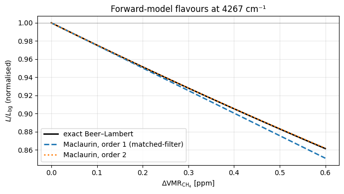
The three curves agree to within a fraction of a percent up to ~0.2 ppm, after which the exact Beer–Lambert model bends below the linear approximation. Order-2 Maclaurin tracks the nonlinear curve to ~0.5 ppm. Beyond that the expansions diverge quickly — but 0.5 ppm is already several times larger than the per-pixel enhancement in a typical oil-and-gas leak, so the matched filter’s linear assumption is safe in the ordinary regime.

3. Synthetic multispectral instrument and SRF¶

InstrumentSpec describes a two-band Gaussian-SRF instrument patterned on Sentinel-2 B11/B12 (but nothing in the radtran package is S2-specific — swap in measured SRFs via SpectralResponseFunction(srf_type='custom', custom_srfs=...)).

instrument = InstrumentSpec(
    name="SWIR-2band-toy",
    band_centers_nm=np.array([1610.0, 2190.0]),
    band_widths_nm=np.array([90.0, 180.0]),  # FWHM for gaussian
    band_names=("B11", "B12"),
    srf_type="gaussian",
)
# SRF on the LUT wavelength grid (sort ascending for the SRF internal ordering).
wl_ascending = np.sort(wl_grid)
srf = instrument.make_srf(wl_ascending)

fig, ax = plt.subplots(figsize=(7, 3))
for b in range(srf.n_bands):
    ax.plot(srf.wavelengths_hr_nm, srf.matrix[b], label=instrument.band_names[b])
ax.set_xlabel("Wavelength [nm]")
ax.set_ylabel("Normalised response")
ax.set_title(f"Instrument SRF — {instrument.name}")
ax.legend()
ax.grid(alpha=0.3)
plt.tight_layout()
plt.show()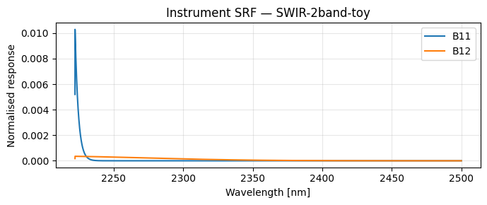

4. Normalised-brightness LUT¶

The nB-LUT pre-tabulates, for each band,

\mathrm{nB}_b(\Delta X) \;=\; \frac{\int f_b(\lambda)\, \exp\!\bigl[-\mathrm{AMF}\cdot\sigma(\lambda)\cdot\Delta X\bigr]\,d\lambda}{\int f_b(\lambda)\,d\lambda}\,, \qquad \Delta X \in [0, X_\text{max}]\ \text{mol/m}^2.

(1)

Per-pixel injection is then nB_b(ΔX_map) — one linear interpolation per pixel per band, irrespective of how many wavenumber points the underlying σ(ν) LUT has.

nb_lut = build_nb_lut(
    ch4_lut,
    srf,
    T_K=T_K,
    p_atm=p_atm,
    amf=geom.air_mass_factor,
    max_delta_column=50.0,
    n_grid=2001,
)
print(
    f"nB LUT: {nb_lut.n_bands} bands × {nb_lut.n_delta} ΔX points "
    f"(0 to {nb_lut.delta_column[-1]:.0f} mol/m²)"
)

fig, ax = plt.subplots(figsize=(7, 4))
for b, name in enumerate(nb_lut.band_names):
    ax.plot(nb_lut.delta_column, nb_lut.nB[b], label=name)
ax.set_xlabel(r"$\Delta X$ [mol/m²]")
ax.set_ylabel(r"$nB_b$ (band-integrated)")
ax.set_title("Normalised-brightness LUT")
ax.legend()
ax.grid(alpha=0.3)
plt.tight_layout()
plt.show()

nB LUT: 2 bands × 2001 ΔX points (0 to 50 mol/m²)

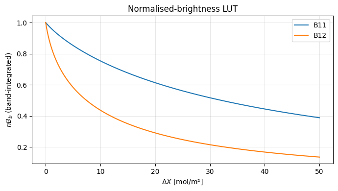
B12 absorbs noticeably more than B11 — consistent with the 2190 nm window overlapping the stronger CH $_4$ $\nu_3$ Q-branch.

5. Plume injection into a synthetic scene¶

Build a Gaussian plume column map via gauss_plume.simulate_plume, then inject into a clean, unit-reflectance two-band scene. In a real pipeline this scene would be a radiance-rescaled Sentinel-2 tile; the injection mathematics (multiply clean B11/B12 by the band-integrated nB factor) is identical.

plume_ds = simulate_plume(
    emission_rate=10.0,  # kg/s ≈ 36000 kg/hr — strong for visibility
    source_location=(0.0, 0.0, 2.0),
    wind_speed=3.0,
    wind_direction=270.0,  # wind from the west → plume east
    stability_class="D",
    domain_x=(-200.0, 400.0, 121),
    domain_y=(-150.0, 150.0, 61),
    domain_z=(0.0, 50.0, 11),
)
# Convert column-integrated mass [kg/m²] → CH4 column in mol/m² (16 g/mol).
M_CH4 = 16.04e-3  # kg/mol
delta_X = plume_ds["column_concentration"].values / M_CH4
# gauss_plume returns a (x, y) field — rename to (ny, nx) for image-style plotting.
delta_X_map = delta_X.T  # (y, x)
print(f"ΔX map shape: {delta_X_map.shape}, peak {delta_X_map.max():.2f} mol/m²")

# Pretend clean scene: flat unit reflectance over B11 + B12.
ny, nx = delta_X_map.shape
clean_scene = np.ones((2, ny, nx), dtype=float)
dirty_scene = inject_plume(clean_scene, delta_X_map, nb_lut)


# Pick colour limits from the actual injected field so the plume is visible
# without clipping. Each band gets its own range because B11 absorbs less.
def _plume_limits(img):
    vmin = float(img.min())
    # Widen a hair above 1.0 so the background stripe is clearly "unity".
    return vmin, 1.005


fig, axes = plt.subplots(1, 4, figsize=(16, 3.5))
im0 = axes[0].imshow(delta_X_map, origin="lower", cmap="viridis")
axes[0].set_title(r"$\Delta X$ [mol/m²]")
fig.colorbar(im0, ax=axes[0], fraction=0.046)

vmin_b11, vmax_b11 = _plume_limits(dirty_scene[0])
im1 = axes[1].imshow(
    dirty_scene[0], origin="lower", cmap="gray", vmin=vmin_b11, vmax=vmax_b11
)
axes[1].set_title(f"B11 (clean × nB) — vmin={vmin_b11:.3f}")
fig.colorbar(im1, ax=axes[1], fraction=0.046)

vmin_b12, vmax_b12 = _plume_limits(dirty_scene[1])
im2 = axes[2].imshow(
    dirty_scene[1], origin="lower", cmap="gray", vmin=vmin_b12, vmax=vmax_b12
)
axes[2].set_title(f"B12 (clean × nB) — vmin={vmin_b12:.3f}")
fig.colorbar(im2, ax=axes[2], fraction=0.046)

ratio = dirty_scene[1] / dirty_scene[0]
vr = max(abs(ratio.min() - 1.0), abs(ratio.max() - 1.0))
im3 = axes[3].imshow(ratio, origin="lower", cmap="RdBu_r", vmin=1 - vr, vmax=1 + vr)
axes[3].set_title("B12 / B11 ratio")
fig.colorbar(im3, ax=axes[3], fraction=0.046)
for ax in axes:
    ax.set_xticks([])
    ax.set_yticks([])
plt.tight_layout()
plt.show()

ΔX map shape: (61, 121), peak 29.76 mol/m²

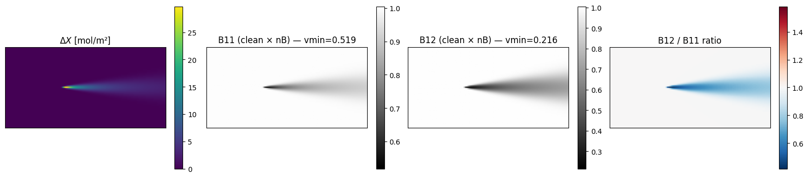
The B12/B11 ratio plot is how classical matched-filter retrievals surface the plume footprint: methane absorbs more strongly in B12 than B11 so the ratio dips below 1 inside the plume. In notebook 05 we replace the visual check with a quantitative matched-filter retrieval that estimates the per-pixel column enhancement.

6. `lookup_nb` directly — diagnostic view¶

inject_plume is a thin wrapper around lookup_nb + multiplication. The lookup itself is useful standalone for diagnostics: the per-band nB map shows where each band “sees” the plume most strongly.

nb_map = lookup_nb(delta_X_map, nb_lut)
fig, axes = plt.subplots(1, 2, figsize=(10, 3.5))
for b, name in enumerate(nb_lut.band_names):
    # Per-band vmin from the actual range; makes the plume visible without clipping.
    vmin = float(nb_map[b].min())
    im = axes[b].imshow(nb_map[b], origin="lower", cmap="magma_r", vmin=vmin, vmax=1.0)
    axes[b].set_title(f"nB_{name} (min {vmin:.3f})")
    axes[b].set_xticks([])
    axes[b].set_yticks([])
    fig.colorbar(im, ax=axes[b], fraction=0.046)
plt.tight_layout()
plt.show()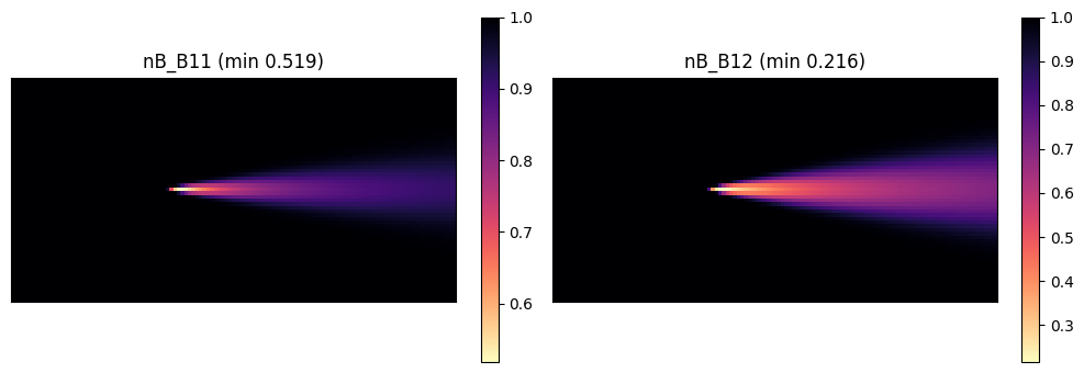

Both bands drop below 1 where the plume is dense, but the B12 dip is sharper. The next notebook uses this asymmetry to quantify $\Delta X$ via a matched-filter retrieval.