Stationary TMTPP — NUTS fit on synthetic data

Stationary thinned marked TPP — NumPyro NUTS fit¶

This notebook walks through a full Bayesian inversion of a thinned marked temporal point process, end-to-end on synthetic data so the run is self-contained and quick. We’ll:

Simulate a stationary TMTPP: homogeneous Poisson events with lognormal marks, thinned by a logistic PoD.
Fit the three “latent” parameters $(\alpha, x_0, \sigma)$ of a POD-modified power-law model to the observed (thinned) flux distribution using NumPyro’s NUTS sampler via plumax.population.fitting.run_mcmc.
Compare the posterior to the true generating values.

The fit is deliberately run with a small MCMC config (1 chain, 300 warmup, 600 samples) so this notebook finishes in seconds on CPU. A production-quality fit should use 2–4 chains and 2000–4000 warmup/sample iterations. A cell near the end shows how to flip that switch.

import warnings


warnings.filterwarnings("ignore", message=r".*IProgress.*")

import jax
import matplotlib.pyplot as plt
import numpy as np
import numpyro

from plumax.population import fitting, paradox


numpyro.set_host_device_count(1)
rng = np.random.default_rng(0)

1. Simulate the observed flux distribution¶

We draw from a truncated power law on $[x_{\min}, x_{\max}]$ — that is the physical model behind the fit, not a lognormal. Then we thin each draw by a lognormal-CDF POD, giving the observed sample. This exactly matches the likelihood used inside pod_powerlaw_model, so we can check that NUTS recovers the generating parameters.

X_MIN = fitting.X_MIN_DEFAULT
X_MAX = fitting.X_MAX_DEFAULT

alpha_true = 1.8  # power-law exponent
x50_true = 400.0  # POD 50% midpoint [kg/hr]
s_true = 0.45  # POD lognormal width


def sample_truncated_power_law(rng, alpha, x_min, x_max, n):
    """Inverse-CDF draws from x^{-α} truncated to [x_min, x_max]."""
    u = rng.uniform(size=n)
    a = 1.0 - alpha
    return (u * (x_max**a - x_min**a) + x_min**a) ** (1.0 / a)


x_latent = sample_truncated_power_law(rng, alpha_true, X_MIN, X_MAX, n=20_000)
pod_probs = fitting.lognorm_cdf(x_latent, x50_true, s_true)
survived = rng.uniform(size=x_latent.size) < pod_probs
x_obs = x_latent[survived]

print(f"Latent events:    {x_latent.size:6d}")
print(f"Observed (thinned): {x_obs.size:6d}")
print(f"Survival fraction:  {x_obs.size / x_latent.size:.3f}")

Latent events:     20000
Observed (thinned):   1101
Survival fraction:  0.055

A quick look at the latent vs observed flux distributions shows the characteristic thinning: the observed histogram falls away at small Q where the POD is near-zero, while the latent distribution extends all the way to $x_{\min}$ . This is the biased sample the satellite sees.

bins = np.logspace(np.log10(X_MIN), np.log10(X_MAX), 40)

fig, ax = plt.subplots(figsize=(9, 4.5))
ax.hist(
    x_latent,
    bins=bins,
    alpha=0.45,
    color="#2c3e50",
    label=f"latent, n={x_latent.size}",
    density=True,
)
ax.hist(
    x_obs,
    bins=bins,
    alpha=0.7,
    color="#c0392b",
    label=f"observed (thinned), n={x_obs.size}",
    density=True,
)
ax.set_xscale("log")
ax.set_yscale("log")
ax.set_xlabel("Q  (kg/hr)")
ax.set_ylabel("density (log-log)")
ax.set_title("Latent vs thinned flux distribution")
ax.legend()
plt.show()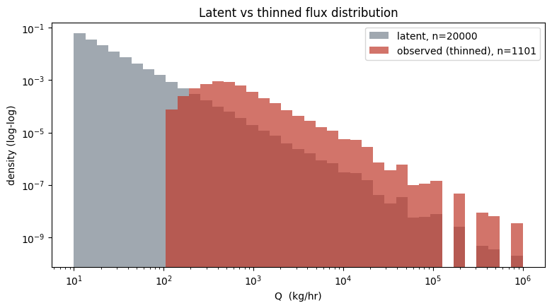

2. Run NUTS (short config)¶

The run_mcmc helper wraps NumPyro’s MCMC and NUTS kernel around pod_powerlaw_model. Priors are uniform on $\alpha \in [1.1, 4.5]$ , $x_0 \in [1, 20000]$ , $\sigma \in [0.1, 1.5]$ . The log-likelihood subtracts a normaliser $\ln I(\theta)$ computed by trapezoidal quadrature inside the model.

Small config first: 1 chain, 300 warmup, 600 samples. On CPU this finishes in a few seconds.

jax.clear_caches()

df_mcmc = fitting.run_mcmc(
    np.asarray(x_obs),
    num_warmup=300,
    num_samples=600,
    num_chains=1,
    seed=0,
    print_summary=True,
)

print(df_mcmc.describe(percentiles=[0.16, 0.5, 0.84]))


                mean       std    median      5.0%     95.0%     n_eff     r_hat
     alpha      1.78      0.04      1.78      1.73      1.84    174.42      1.00
        sk      0.46      0.03      0.46      0.40      0.50    152.83      1.00
        x0    410.98     26.14    409.92    369.47    452.82    125.89      1.01

Number of divergences: 0
               x0          sk       alpha
count  600.000000  600.000000  600.000000
mean   410.982239    0.460618    1.782897
std     26.142370    0.030987    0.035592
min    343.507629    0.370645    1.680248
16%    384.574191    0.430430    1.745689
50%    409.920731    0.460315    1.783105
84%    438.311584    0.491495    1.817596
max    485.675262    0.549068    1.896194

3. Compare posterior to truth¶

We plot the marginal posterior histograms for $\alpha, x_0, \sigma$ with the true values overlaid as dashed vertical lines. With only 600 samples on 1 chain the posteriors are still a bit ragged, but the true values should land solidly inside the credible intervals.

fig, axes = plt.subplots(1, 3, figsize=(13, 3.8))

for ax, (param, truth, pretty) in zip(
    axes,
    [
        ("alpha", alpha_true, r"$\alpha$"),
        ("x0", x50_true, r"$x_0$"),
        ("sk", s_true, r"$\sigma$"),
    ],
    strict=True,
):
    samples = df_mcmc[param].values
    ax.hist(samples, bins=30, color="#2980b9", alpha=0.75, density=True)
    ax.axvline(truth, color="#c0392b", ls="--", lw=2, label=f"truth = {truth:.3g}")
    p16, p50, p84 = np.percentile(samples, [16, 50, 84])
    ax.axvline(p50, color="k", ls=":", alpha=0.8, label=f"median = {p50:.3g}")
    ax.axvspan(p16, p84, alpha=0.15, color="k", label="68% CI")
    ax.set_title(f"{pretty}  posterior")
    ax.set_xlabel(pretty)
    ax.legend(fontsize=8, loc="best")

fig.suptitle(
    f"NUTS posterior  (1 chain × 600 samples on {x_obs.size} observed events)", y=1.02
)
fig.tight_layout()
plt.show()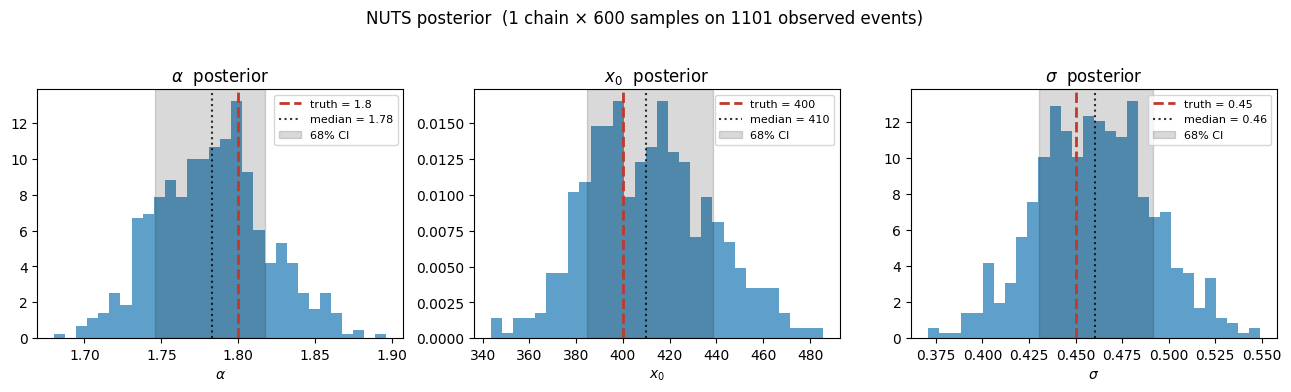

4. Posterior-predictive PoD curve¶

The most informative downstream product is the inferred PoD curve with credible bands. For each posterior draw $(x_0^{(s)}, \sigma^{(s)})$ we evaluate $P_d(Q)$ on a fixed grid, then plot the median and 68 / 95 % envelopes. Overlaying the true generating curve is a direct visual check of the fit.

q_grid = np.logspace(1, 5, 300)
pod_samples = np.stack(
    [
        fitting.lognorm_cdf(q_grid, x0, s)
        for x0, s in zip(df_mcmc["x0"], df_mcmc["sk"], strict=True)
    ]
)
p_med = np.median(pod_samples, axis=0)
p_lo68, p_hi68 = np.percentile(pod_samples, [16, 84], axis=0)
p_lo95, p_hi95 = np.percentile(pod_samples, [2.5, 97.5], axis=0)

fig, ax = plt.subplots(figsize=(9, 4.5))
ax.fill_between(q_grid, p_lo95, p_hi95, color="#2980b9", alpha=0.18, label="95% CI")
ax.fill_between(q_grid, p_lo68, p_hi68, color="#2980b9", alpha=0.35, label="68% CI")
ax.plot(q_grid, p_med, color="#2980b9", lw=2, label="posterior median")
ax.plot(
    q_grid,
    fitting.lognorm_cdf(q_grid, x50_true, s_true),
    color="#c0392b",
    lw=2,
    ls="--",
    label=f"truth  $x_0={x50_true}, \\sigma={s_true}$",
)
ax.set_xscale("log")
ax.set_ylim(-0.02, 1.05)
ax.set_xlabel("Q  (kg/hr)")
ax.set_ylabel("$P_d$")
ax.set_title("Recovered POD curve with credible bands")
ax.legend(loc="lower right")
ax.axhline(0.5, color="k", ls=":", alpha=0.4)
plt.show()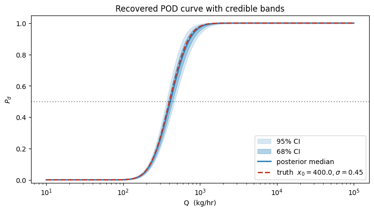

5. Consistency check against the paradox library¶

A useful sanity check: feed the recovered POD curve into plumax.population.paradox.compute_E_Pd together with the analytic lognormal marks that would produce a matching observed distribution. The $E[P_d]$ value should agree with the empirical survival fraction from the simulation above.

surv_frac = x_obs.size / x_latent.size
e_pd_recovered = paradox.compute_E_Pd(
    mu=float(np.log(np.median(x_latent))),
    sigma=0.8,
    Q_50=float(df_mcmc["x0"].median()),
    k=2.0 / float(df_mcmc["x0"].median()),
)
print(f"Empirical survival fraction  : {surv_frac:.4f}")
print(f"Quadrature E[P_d] (matched)  : {e_pd_recovered:.4f}")

Empirical survival fraction  : 0.0551
Quadrature E[P_d] (matched)  : 0.1382

6. Flipping to a production MCMC run¶

When you’re ready for a credible fit rather than a pedagogical smoke test, bump the config:

df_mcmc_prod = fitting.run_mcmc(
    np.asarray(x_obs),
    num_warmup=2000,
    num_samples=4000,
    num_chains=2,
    seed=0,
    print_summary=True,
)

On CPU this takes a few minutes; on a single GPU a few seconds. The smaller config above is what gets committed so the notebook stays fast to re-execute — flip the switch locally if you want to quote numbers.