Plume vetting: a spectral test for matched-filter candidates

The matched filter scores each pixel by one projection of its spectrum, so anything that removes light under methane’s 2.3 μm band scores: carbonate soils, salt pans, shadows, striping. Plume vetting (Xiang et al. 2024; Růžička et al. 2026) goes back to the radiances. It pairs a candidate’s strongest pixels with pixels outside it that have the same surface, divides them, and fits methane’s transmittance times a smooth continuum to the ratio; the misfit $D_{\text{norm}}$ accepts or rejects the candidate. This notebook builds one EMIT-like scene in which the matched filter scores a carbonate patch above a real plume, and vets both.

The work comes from two packages. plumax.vetting works on plume candidates: their seeds and background pool, the null over the plume’s shape, and one call that vets a candidate. radtrax’s radtrax.retrieval.absorption is the plume-agnostic absorption-shape test those pieces run: the gas’s window and transmittance, the pairing of two pixel sets, the ratio, the fit and $D_{\text{norm}}$ . Every function below is imported from one of the two; the theory is on the plume vetting page.

What you’ll learn:

How to get the transmittance the fit needs from radtrax’s ForwardModel, and why a constant absorption coefficient biases the column low.
How seeds, one-to-one pairing and the ratio spectrum cancel the surface.
How the profile fit and $D_{\text{norm}}$ separate a plume from a confounder, and how a null from the same scene calibrates the score.

Background¶

For a pixel under a plume and a pixel outside it with the same surface, sun and atmosphere, the ratio of their radiances cancels everything but the plume and what the two surfaces do not share:

R(\lambda) = \frac{\overline{L_{\text{in}}}(\lambda)}{\overline{L_{\text{out}}}(\lambda)} \approx P(\lambda; c)\, E(\lambda; \Delta X), \qquad E_b(\Delta X) = \frac{y_b(\text{state} + \Delta X)}{y_b(\text{state})}

(1)

with $E$ methane’s band transmittance for a column enhancement $\Delta X$ [mol/m²] and $P$ a low-order Legendre series that absorbs the surface mismatch. The fit gives $\widehat{\Delta X}$ , and the score divides out the continuum, $q = R / P$ , and compares $q$ with $E$ relative to $q$ ’s own spread:

D_{\text{norm}} = \frac{\operatorname{mean}_\lambda \lvert q - E(\widehat{\Delta X}) \rvert}{\operatorname{mean}_\lambda \lvert q - \bar q \rvert}

(2)

A perfect fit gives 0; no methane gives $\widehat{\Delta X} = 0$ , $E = 1$ and $D_{\text{norm}} \approx 1$ . EMIT’s daily digest alerts below 0.3.

import subprocess
import sys


try:
    import google.colab  # noqa: F401

    IN_COLAB = True
except ImportError:
    IN_COLAB = False

if IN_COLAB:
    subprocess.run(
        [
            sys.executable,
            "-m",
            "pip",
            "install",
            "-q",
            "plumax @ git+https://github.com/jejjohnson/plumax@main",
        ],
        check=True,
    )

import warnings


warnings.filterwarnings("ignore", message=r".*IProgress.*")

import jax


jax.config.update("jax_enable_x64", True)

import matplotlib.pyplot as plt
import numpy as np
import radtrax
from radtrax.atmosphere import (
    AVOGADRO_PER_MOL,
    BOLTZMANN_J_PER_K,
    ViewingGeometry,
    afgl_us_standard,
)
from radtrax.instrument import GaussianInstrument
from radtrax.retrieval.absorption import (
    AbsorptionWindow,
    fit_transmittance,
    pair_pixels,
    transmittance_table,
)
from radtrax.retrieval.matched_filter import apply_image, estimate_cov_shrunk
from radtrax.solvers import BeerLambert
from radtrax.spectroscopy import TableOpacity
from radtrax.spectroscopy.synthetic import NU_CM, synthetic_table
from radtrax.surface import Lambertian
from scipy.ndimage import gaussian_filter

from plumax.vetting import (
    background_pool,
    null_masks,
    null_pvalue,
    select_seeds,
    vet_candidate,
)

import importlib.util


try:
    from IPython import get_ipython

    ipython = get_ipython()
except ImportError:
    ipython = None

if ipython is not None and importlib.util.find_spec("watermark") is not None:
    ipython.run_line_magic("load_ext", "watermark")
    ipython.run_line_magic(
        "watermark", "-v -m -p numpy,scipy,jax,equinox,radtrax,plumax"
    )
else:
    print("watermark extension not installed; skipping reproducibility readout.")

Python implementation: CPython
Python version       : 3.13.17
IPython version      : 9.10.0

numpy  : 2.4.6
scipy  : 1.17.1
jax    : 0.11.0
equinox: 0.13.8
radtrax: 0.0.0
plumax : 0.1.2

Compiler    : Clang 23.1.3 
OS          : Linux
Release     : 6.18.44-fc-v165
Machine     : x86_64
Processor   : x86_64
CPU cores   : 2
Architecture: 64bit

1. The transmittance the fit needs¶

Nine EMIT-like bands (8.5 nm wide, every 7.5 nm, 2296–2356 nm) on radtrax · 3’s synthetic table of 150 Voigt lines, so the notebook runs without HITRAN. The model is AFGL US Standard to 20 km with CH₄ and a stand-in H₂O, a 35° sun and a 10° view. radtrax’s transmittance_table puts a column enhancement $\Delta X$ in the bottom layer and divides by the plume-free radiance; linear=True gives the reference code’s older model, $\exp(-\varepsilon \Delta X)$ with $\varepsilon = -\partial \ln y / \partial \Delta X$ at 0, which is the matched filter’s target from radtrax’s unit_absorption_target.

CENTERS_NM = np.arange(2296.0, 2357.0, 7.5)  # (B,) = (9,)
opacity = TableOpacity.from_datasets(
    {"CH4": synthetic_table(seed=0), "H2O": synthetic_table(seed=1)}
)
instrument = GaussianInstrument(NU_CM, CENTERS_NM, np.full(CENTERS_NM.size, 8.5))
model = radtrax.ForwardModel(opacity, BeerLambert(), instrument)
state = afgl_us_standard(z_top_km=20.0, gases=["CH4", "H2O"])
geometry = ViewingGeometry.from_angles(35.0, 10.0)
DELTA_GRID = np.linspace(0.0, 0.4, 801)  # ΔX [mol/m²]                         (D,)

# 1 ppm·m at the surface layer, in mol/m², for quoting columns as EMIT does
n_air = float(state.p_pa[0] / (BOLTZMANN_J_PER_K * state.t_k[0]))  # molecules/m³
PPMM = 1e-6 * n_air / AVOGADRO_PER_MOL
print(f"1 ppm·m = {PPMM:.3e} mol/m² at the surface layer")

1 ppm·m = 4.030e-05 mol/m² at the surface layer

The table is computed in 8 chunks of about 100 columns, each with its own background run at $\Delta X = 0$ : one pass over all 801 holds several GB of per-layer, per-wavenumber intermediates on the 14,000-wavenumber grid. A fit of the exact transmittance with a constant coefficient returns too small a column, because lines saturate: a strong plume absorbs less per molecule than the weak-absorption slope predicts.

chunks = [
    np.asarray(transmittance_table(model, state, geometry, c))
    for c in np.array_split(DELTA_GRID, 8)
]
E_TABLE = np.concatenate(chunks)  # (D, B)
E_LIN = transmittance_table(model, state, geometry, DELTA_GRID, linear=True)
eps = -np.log(np.asarray(E_LIN[1])) / DELTA_GRID[1]  # ε [m²/mol]           (B,)
for dx in (0.05, 0.1, 0.3):
    E_exact = E_TABLE[np.argmin(np.abs(DELTA_GRID - dx))]
    dx_lin = -(eps @ np.log(E_exact)) / (eps @ eps)
    print(
        f"ΔX = {dx:.2f} mol/m² ({dx / PPMM:,.0f} ppm·m): constant ε gives "
        f"{100 * (dx_lin / dx - 1):+.1f} %"
    )
deepest = 1 - float(E_TABLE[np.searchsorted(DELTA_GRID, 0.1)].min())
print(f"deepest band absorption at 0.1 mol/m²: {100 * deepest:.1f} %")

ΔX = 0.05 mol/m² (1,241 ppm·m): constant ε gives -1.4 %
ΔX = 0.10 mol/m² (2,481 ppm·m): constant ε gives -2.8 %
ΔX = 0.30 mol/m² (7,444 ppm·m): constant ε gives -7.7 %
deepest band absorption at 0.1 mol/m²: 1.8 %

2. The scene and the matched filter¶

A 64 × 64 scene: 30 channels outside methane’s band (1000–2050 nm) that carry only the surface, and the 9 absorbing bands. Three surface classes in patches, with a brightness texture of a few percent. Candidate A is a Gaussian plume from a point source; its mask is where the truth exceeds about 500 ppm·m. Candidate B is a plume-shaped ellipse of a carbonate-like surface whose reflectance dips by 6 % around 2335 nm. Gaussian noise at SNR 300 per channel. Radiance is reflectance times the unit-albedo forward model, $L_b = \rho_b\, y_b(0)\, E_b(\Delta X)$ , interpolated in $\Delta X$ from the table.

rng = np.random.default_rng(0)
H = W = 64
WL_OUT = np.linspace(1000.0, 2050.0, 30)
WL = np.concatenate([WL_OUT, CENTERS_NM])  # (B,) = (39,)
IN = np.arange(WL_OUT.size, WL.size)

field = gaussian_filter(rng.standard_normal((H, W)), 6.0)
cls = np.digitize(field, np.quantile(field, [1 / 3, 2 / 3]))  # (H, W)
coef = np.array([[0.28, 0.06, -0.04], [0.18, 0.08, -0.04], [0.40, -0.03, -0.02]])
x_wl = (WL - 1700.0) / 700.0
rho_cls = coef @ np.stack([np.ones_like(x_wl), x_wl, x_wl**2])  # (3, B)
bright = 1 + 0.5 * gaussian_filter(rng.standard_normal((H, W)), 2.0)
rho = rho_cls[cls] * bright[..., None]  # (H, W, B)

ii, jj = np.mgrid[:H, :W]
along = jj - 14.0
sigma_y = 1.5 + 0.18 * np.clip(along, 0, None)
plume = 0.20 * np.exp(-((ii - 40.0) ** 2) / (2 * sigma_y**2)) * 1.5 / sigma_y
delta_x = np.where(along > 0, plume, 0.0)
delta_x += 0.20 * np.exp(-((ii - 40.0) ** 2 + (jj - 14.0) ** 2) / 2.0)
mask_a = delta_x > 0.02

u, v = jj - 44.0, ii - 16.0
ang = np.deg2rad(25.0)
ellipse = ((u * np.cos(ang) + v * np.sin(ang)) / 11.0) ** 2
ellipse += ((-u * np.sin(ang) + v * np.cos(ang)) / 3.2) ** 2
mask_b = ellipse < 1
dip = 1 - 0.06 * np.exp(-((WL - 2335.0) ** 2) / (2 * 15.0**2))  # (B,)

y0 = np.asarray(model(state, Lambertian(1.0), geometry))  # plume-free (B,)
E_pix = np.stack(
    [np.interp(delta_x.ravel(), DELTA_GRID, E_TABLE[:, b]) for b in range(IN.size)],
    -1,
).reshape(H, W, IN.size)
L_true = np.empty((H, W, WL.size))
L_true[..., : WL_OUT.size] = rho[..., : WL_OUT.size] * y0.mean() * (2300 / WL_OUT) ** 2
L_true[..., IN] = rho[..., IN] * y0 * E_pix
L_true[mask_b] *= dip
L = L_true * (1 + rng.standard_normal(L_true.shape) / 300.0)
masks = np.stack([mask_a, mask_b])  # (C, H, W)

# matched filter on ln L, target t (zero out of band): ΔX_MF [mol/m²]
lnL = np.log(L)
t = radtrax.unit_absorption_target(model, state, Lambertian(1.0), geometry)
target = np.concatenate([np.zeros(WL_OUT.size), np.asarray(t)])
mu = lnL.reshape(-1, WL.size).mean(0)
mf = np.asarray(apply_image(lnL, mu, estimate_cov_shrunk(lnL, mu), target))
mf_sigma = float(np.std(mf[~masks.any(0)]))
print(f"MF noise off the candidates: {mf_sigma / PPMM:,.0f} ppm·m")
for name, m in (("A", mask_a), ("B", mask_b)):
    print(
        f"{name}: {m.sum()} pixels, mean MF {mf[m].mean() / PPMM:,.0f} ppm·m, "
        f"peak {mf[m].max() / PPMM:,.0f} ppm·m, mean truth "
        f"{delta_x[m].mean() / PPMM:,.0f} ppm·m"
    )

MF noise off the candidates: 484 ppm·m
A: 748 pixels, mean MF 593 ppm·m, peak 7,135 ppm·m, mean truth 1,035 ppm·m
B: 111 pixels, mean MF 1,162 ppm·m, peak 2,555 ppm·m, mean truth 11 ppm·m

fig, axes = plt.subplots(1, 2, figsize=(12, 5))
for ax, (title, im) in zip(
    axes, (("true ΔX", delta_x), ("matched filter", mf)), strict=True
):
    h = ax.imshow(im / PPMM, cmap="RdBu_r", vmin=-3000, vmax=3000)
    ax.contour(mask_a, levels=[0.5], colors="C2")
    ax.contour(mask_b, levels=[0.5], colors="C1")
    ax.set_title(title)
    ax.set_xticks([])
    ax.set_yticks([])
fig.colorbar(h, ax=axes, shrink=0.8, label="ppm·m")
axes[0].text(2, 60, "A plume", color="C2")
axes[0].text(34, 6, "B carbonate", color="C1")
plt.show()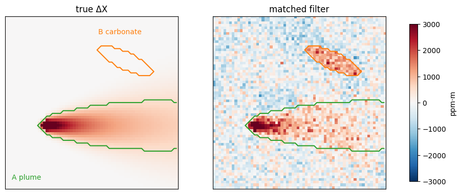

The matched filter flags both, and scores the carbonate patch B higher on average than the plume A, whose mask includes the faint tail.

3. Vetting the two candidates¶

radtrax’s AbsorptionWindow here fits the nine absorbing bands and pairs on the 30 others. vet_candidate takes the seeds (select_seeds), the background pool (background_pool: every pixel within 16 pixels of the seeds’ bounding box, outside both candidates, with a matched-filter score under twice its noise), pairs the two sets one to one with radtrax’s pair_pixels, and fits the ratio.

window = AbsorptionWindow(
    "CH4",
    fit_nm=((2290.0, 2360.0),),
    absorbing_nm=((2290.0, 2360.0),),
    mf_background_mol_m2=2 * mf_sigma,
)
results = {}
for name, m in (("A", mask_a), ("B", mask_b)):
    results[name] = vet_candidate(
        L, mf, m, WL, E_TABLE, DELTA_GRID, window, exclude=masks, box=16
    )
    r = results[name]
    print(
        f"{name}: ΔX̂ = {float(r.delta) / PPMM:,.0f} ppm·m, "
        f"D_norm = {float(r.d_norm):.2f}, {r.n_pairs} pairs"
    )

A: ΔX̂ = 1,741 ppm·m, D_norm = 0.14, 64 pairs

B: ΔX̂ = 0 ppm·m, D_norm = 1.00, 54 pairs

A fits as methane with $D_{\text{norm}}$ well below 0.3. B fits at $\widehat{\Delta X} = 0$ : the continuum takes the carbonate’s smooth dip, nothing methane-shaped is left, and $D_{\text{norm}} \approx 1$ . A’s column is below the truth over its seed pixels for two reasons: the fit returns the column of the mean transmittance, not the mean column (the transmittance is convex in $\Delta X$ ), and paired surfaces never match exactly.

seeds_a = select_seeds(mf, mask_a)
pool_a = background_pool(
    mf, seeds_a, threshold=window.mf_background_mol_m2, exclude=masks, box=16
)
i_in, _ = pair_pixels(
    L, np.flatnonzero(seeds_a), np.flatnonzero(pool_a), window.pairing_bands(WL)
)
truth_a = delta_x.ravel()[i_in].mean()
print(
    f"A: truth over its kept pixels {truth_a / PPMM:,.0f} ppm·m; the fit recovers "
    f"{100 * float(results['A'].delta) / truth_a:.0f} %"
)
fit_lin = fit_transmittance(results["A"].ratio, E_LIN, DELTA_GRID, CENTERS_NM)
print(f"A with a constant coefficient: {float(fit_lin.delta) / PPMM:,.0f} ppm·m")

A: truth over its kept pixels 1,865 ppm·m; the fit recovers 93 %
A with a constant coefficient: 1,691 ppm·m

4. A null from the same scene¶

The honest null is this scene’s clutter with no plume. null_masks draws 100 copies of each mask, rotated and translated off both candidates; each is vetted exactly as the candidate, and null_pvalue gives $\hat p$ , the fraction that score at or below it.

key = jax.random.key(0)
null_scores = {}
for name, m in (("A", mask_a), ("B", mask_b)):
    key, sub = jax.random.split(key)
    copies = null_masks(m, 100, key=sub, exclude=masks)
    null_scores[name] = np.array(
        [
            float(
                vet_candidate(
                    L, mf, c, WL, E_TABLE, DELTA_GRID, window, exclude=masks, box=16
                ).d_norm
            )
            for c in copies
        ]
    )
    p_hat = null_pvalue(float(results[name].d_norm), null_scores[name])
    q05, q50 = np.quantile(null_scores[name], [0.05, 0.5])
    print(
        f"{name}: p̂ = {p_hat:.2f}; null D_norm 5th percentile {q05:.2f}, "
        f"median {q50:.2f}, {int((null_scores[name] < 0.3).sum())} of 100 below 0.3"
    )

A: p̂ = 0.00; null D_norm 5th percentile 0.47, median 0.79, 0 of 100 below 0.3

B: p̂ = 0.45; null D_norm 5th percentile 0.49, median 1.00, 1 of 100 below 0.3

fig, axes = plt.subplots(2, 2, figsize=(12, 8))
for row, name in enumerate(("A", "B")):
    r = results[name]
    ax = axes[row, 0]
    ax.scatter(
        CENTERS_NM,
        r.ratio / r.fit.continuum,
        color=f"C{2 - row}",
        label="R / P (observed)",
    )
    ax.plot(CENTERS_NM, r.fit.transmittance, "k--", label="E(ΔX̂) (fit)")
    ax.set_title(
        f"{name}: ΔX̂ = {float(r.delta) / PPMM:,.0f} ppm·m, "
        f"D_norm = {float(r.d_norm):.2f}"
    )
    ax.set_xlabel("wavelength (nm)")
    ax.set_ylabel("transmittance")
    ax.legend()
    ax = axes[row, 1]
    ax.hist(null_scores[name], bins=np.linspace(0, 1.3, 27), color="0.7")
    ax.axvline(float(r.d_norm), color=f"C{2 - row}", lw=2)
    ax.axvline(0.3, color="k", ls="--", lw=1)
    ax.set_title(f"{name}: D_norm of 100 null copies (dashed: 0.3)")
    ax.set_xlabel("D_norm")
fig.tight_layout()
plt.show()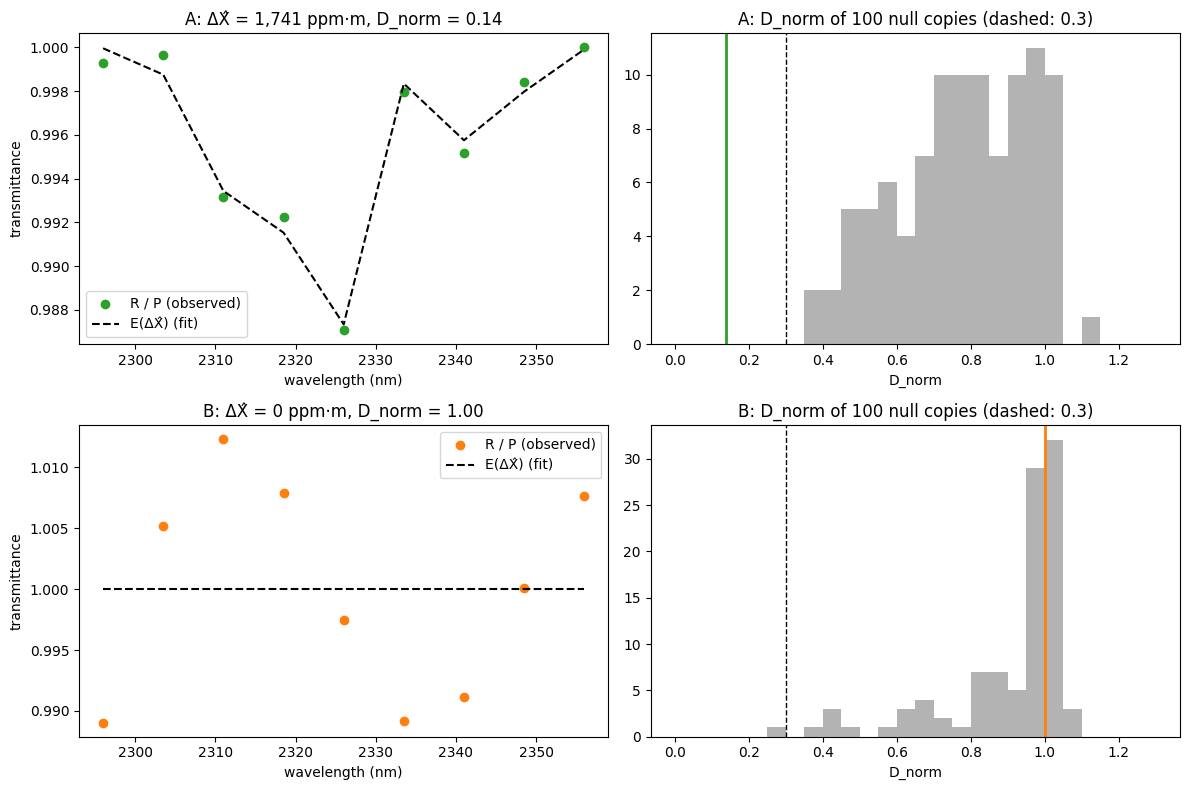

Summary¶

The matched filter scored the carbonate patch above the plume; the spectral fit reversed the order, accepting A and finding no methane in B.
The transmittance comes from radtrax’s forward model for the scene’s own geometry and water vapour, so the curve of growth is built in; a constant coefficient biases strong plumes low.
$D_{\text{norm}}$ thresholds depend on the window and the continuum’s degree (this scene has 9 bands, EMIT’s window 46), so report the scene-null $\hat p$ with every score and set the threshold per sensor on real scenes.
Vetting’s $\widehat{\Delta X}$ is a score, not a retrieval: the column for an emission rate comes from a per-pixel retrieval of the vetted plume.