RBIG Walk-Through
![]()
This notebook is a self-contained guide to the Rotation-Based Iterative
Gaussianization (RBIG) algorithm. It covers the theory, the step-by-step
algorithm, and a hands-on demonstration using the composable rbig API.
Contents
Colab / fresh environment? Run the cell below to install
rbigfrom GitHub. Skip if already installed.
!pip install "rbig[all] @ git+https://github.com/jejjohnson/rbig.git" -q
Why Gaussianization?
It is notorious that we say "assume our data is Gaussian". We do this all of the time in practice because Gaussian data has nice properties:
- Closed-form solutions for many statistical quantities
- Linear dependence structure — the covariance matrix captures everything
- Analytical expressions for entropy, KL-divergence, and mutual information
But as sensors get better, data gets bigger, and algorithms get more sophisticated, the Gaussian assumption rarely holds in practice.
What if we could make our data Gaussian? If it were possible, then all of those nice properties would apply — because the data really is Gaussian after the transformation. This is exactly what Gaussianization does: apply a series of invertible transformations to map $\mathcal{X}$ to the Gaussian domain $\mathcal{Z}$.
Gaussianization gives us:
- Process dimensions independently (statistical independence of components)
- Alleviate the curse of dimensionality
- Tackle PDF estimation directly — with a PDF we can sample and assign probabilities
- Apply methods that assume Gaussianity
- Get insight into data characteristics via information-theoretic measures
The Density Destructor View
RBIG belongs to the density destructor family of methods. A density destructor is a generative model that transforms a data distribution $\mathcal{X}$ to a base distribution $\mathcal{Z}$ through an invertible transformation $\mathcal{G}_\theta$:
$$\begin{aligned} x &\sim \mathcal{P}_x \quad (\text{Data Distribution})\\ \hat{z} &= \mathcal{G}_\theta(x) \sim \mathcal{P}_z \quad (\text{Base Distribution}) \end{aligned}$$
Because the transforms are invertible, we can use the change of variables formula to get probability estimates of the original data space:
$$p_x(x) = p_z\!\left(\mathcal{G}_\theta(x)\right) \left|\frac{\partial \mathcal{G}_\theta(x)}{\partial x}\right| = p_z\!\left(\mathcal{G}_\theta(x)\right) \left|\nabla_x \mathcal{G}(x)\right|$$
RBIG vs. Normalizing Flows
If you are familiar with normalizing flows, you'll find similarities. They are inherently the same family of methods. However, most normalizing flows focus on minimizing the log-determinant of the Jacobian as a cost function. RBIG has a different objective: maximize the negentropy (or equivalently minimize the total correlation).
Negentropy measures departure from Gaussianity:
$$J(\mathbf{x}) = H(\mathbf{x}_\text{gauss}) - H(\mathbf{x})$$
where $H(\mathbf{x}_\text{gauss})$ is the entropy of a Gaussian with the same covariance as $\mathbf{x}$. By destroying the density (driving negentropy to zero), we maximize the entropy and remove all redundancies within the marginals. This formulation also allows us to estimate many information- theoretic measures (entropy, MI, KLD) as a by-product.
Historical Context
Gaussianization has been approached via several methods:
- Projection Pursuit — iteratively finds directions that maximize non-Gaussianity
- Marginal Gaussianization — independently transforms each dimension
- RBIG — combines marginal Gaussianization with rotations; more computationally efficient and simpler to implement than the alternatives
Algorithm Overview
Gaussianization — Given a random variable $\mathbf{x} \in \mathbb{R}^d$, a Gaussianization transform is an invertible and differentiable transform $\mathcal{G}(\mathbf{x})$ such that $\mathcal{G}(\mathbf{x}) \sim \mathcal{N}(0, \mathbf{I})$.
The RBIG iteration is:
$$\mathcal{G}: \mathbf{x}^{(k+1)} = \mathbf{R}_{(k)} \cdot \mathbf{\Psi}_{(k)}\!\left(\mathbf{x}^{(k)}\right)$$
where:
- $\mathbf{\Psi}_{(k)}$ is the marginal Gaussianization of each dimension of $\mathbf{x}^{(k)}$ at iteration $k$.
- $\mathbf{R}_{(k)}$ is a rotation matrix applied to the marginally Gaussianized variable.
Repeating these two steps iteratively drives the joint distribution towards a standard multivariate Gaussian.
Marginal Gaussianization ($\Psi$)
To go from any distribution $\mathcal{P}$ to a Gaussian $\mathcal{G}$:
- Estimate the empirical CDF for each feature
- Apply the CDF to obtain a uniform variable $u \in [0, 1]$
- Apply the inverse Gaussian CDF $\Phi^{-1}$ to map to $\mathcal{N}(0,1)$
The pipeline for a single dimension $d$ is:
$$x_d \xrightarrow{F_d} u_d \xrightarrow{\Phi^{-1}} z_d$$
Rotation ($R$)
The rotation must be orthogonal, orthonormal, and invertible. Options include:
- PCA — Principal Components Analysis (default)
- ICA — Independent Components Analysis
- Random — Random orthogonal rotations
The full transformation at each layer:
$$\mathcal{P} \rightarrow \mathcal{U} \rightarrow \mathcal{G} \rightarrow \mathbf{R} \cdot \mathcal{G}$$
%matplotlib inline
import matplotlib.pyplot as plt
import numpy as np

from rbig import AnnealedRBIG, MarginalGaussianize, PCARotation, RBIGLayer

plt.style.use("seaborn-v0_8-paper")
/anaconda/lib/python3.13/site-packages/tqdm/auto.py:21: TqdmWarning: IProgress not found. Please update jupyter and ipywidgets. See https://ipywidgets.readthedocs.io/en/stable/user_install.html
  from .autonotebook import tqdm as notebook_tqdm
def plot_2d_joint(data, title="Data", color="steelblue"):
    _fig, ax = plt.subplots(figsize=(5, 5))
    ax.scatter(data[:, 0], data[:, 1], s=5, alpha=0.5, color=color)
    ax.set_title(title)
    ax.set_xticks([])
    ax.set_yticks([])
    plt.tight_layout()
    plt.show()
Data
We generate a 2-D "sin-wave" dataset — a non-Gaussian joint distribution with visible nonlinear dependence.
seed = 123
rng = np.random.RandomState(seed=seed)

num_samples = 2_000
x = np.abs(2 * rng.randn(1, num_samples))
y = np.sin(x) + 0.25 * rng.randn(1, num_samples)
data = np.vstack((x, y)).T

print(f"Data shape: {data.shape}")
plot_2d_joint(data, title="Original Data")
Data shape: (2000, 2)

Step I — Marginal Gaussianization
We use MarginalGaussianize to transform each feature independently to
approximately standard Gaussian using the empirical CDF + probit.
This is the $\mathbf{\Psi}$ step: for each dimension $d$, we estimate the empirical CDF $F_d$, apply it to get a uniform variable, and then apply $\Phi^{-1}$ to obtain a Gaussian variable.
mg = MarginalGaussianize()
mg.fit(data)
data_mg = mg.transform(data)

plot_2d_joint(data_mg, title="After Marginal Gaussianization", color="darkorange")

After this step each marginal is approximately Gaussian, but the joint distribution still shows dependence (the scatter plot is not circular).
Step II — Rotation (PCA)
We apply PCARotation with whitening to decorrelate the Gaussianized features.
This is the $\mathbf{R}$ step: it mixes the dimensions so that the next round
of marginal Gaussianization can attack the remaining dependence structure.
pca_rot = PCARotation(whiten=True)
pca_rot.fit(data_mg)
data_rot = pca_rot.transform(data_mg)

plot_2d_joint(data_rot, title="After PCA Rotation", color="seagreen")

One RBIG layer (marginal Gaussianization + rotation) has already significantly reduced the dependence. However, for strongly non-Gaussian data we need many layers.
layer = RBIGLayer(
    marginal=MarginalGaussianize(),
    rotation=PCARotation(whiten=True),
)
layer.fit(data)
data_layer = layer.transform(data)

# Verify that RBIGLayer produces a transform with similar statistics
mean_manual = np.mean(data_rot, axis=0)
mean_layer = np.mean(data_layer, axis=0)
cov_manual = np.cov(data_rot, rowvar=False)
cov_layer = np.cov(data_layer, rowvar=False)

np.testing.assert_allclose(mean_layer, mean_manual, rtol=1e-3, atol=1e-3)
np.testing.assert_allclose(cov_layer, cov_manual, rtol=1e-3, atol=1e-3)
print(
    "RBIGLayer output has similar mean and covariance to manual marginal + rotation steps ✓"
)
RBIGLayer output has similar mean and covariance to manual marginal + rotation steps ✓
Inverse transform
RBIGLayer is an invertible transform: we can map the Gaussianized data back
to the original space.
data_reconstructed = layer.inverse_transform(data_layer)
residual = np.abs(data - data_reconstructed).mean()
print(f"Mean absolute reconstruction error: {residual:.4e}")
Mean absolute reconstruction error: 1.0400e-03
Layer Progression
To visualize how the distribution evolves, we show the output after 1, 3, and 5 RBIG layers. With each additional layer the joint distribution becomes more circular (more Gaussian).
import seaborn as sns

n_layer_list = [1, 3, 5]
fig, axes = plt.subplots(1, 3, figsize=(15, 5))

for ax, n in zip(axes, n_layer_list, strict=False):
    model_n = AnnealedRBIG(
        n_layers=n,
        rotation="pca",
        patience=n + 1,  # never stop early in this demo
        random_state=seed,
    )
    Z_n = model_n.fit_transform(data)
    ax.hexbin(Z_n[:, 0], Z_n[:, 1], gridsize=30, cmap="Reds", mincnt=1)
    ax.set_title(f"{n} layer{'s' if n > 1 else ''}")
    ax.set_xticks([])
    ax.set_yticks([])

plt.suptitle("RBIG output at increasing numbers of layers", y=1.01)
plt.tight_layout()
plt.show()

Full RBIG Model with AnnealedRBIG
AnnealedRBIG stacks many RBIGLayer instances and iterates until the total
correlation (TC) converges. Recall that RBIG's objective is to minimize TC —
when TC reaches zero, the data is factorial Gaussian and no more layers are
needed.
rbig_model = AnnealedRBIG(
    n_layers=50,
    rotation="pca",
    patience=10,
    random_state=seed,
)
rbig_model.fit(data)

print(f"Number of layers fitted: {len(rbig_model.layers_)}")
Number of layers fitted: 27
Transformed data
data_gauss = rbig_model.transform(data)
plot_2d_joint(data_gauss, title="After Full RBIG (should be ≈ N(0,1)²)", color="purple")

Total correlation per layer
tc_per_layer_ records the total correlation of the data after each layer.
It should decrease monotonically towards zero as the algorithm drives the data
towards a factorial Gaussian.
fig, ax = plt.subplots()
ax.plot(rbig_model.tc_per_layer_)
ax.set_xlabel("Layer")
ax.set_ylabel("Total Correlation (nats)")
ax.set_title("TC convergence per RBIG layer")
plt.tight_layout()
plt.show()

Inverse transform (reconstruction)
data_inv = rbig_model.inverse_transform(data_gauss)
residual_full = np.abs(data - data_inv).mean()
print(f"Full RBIG mean absolute reconstruction error: {residual_full:.4e}")
Full RBIG mean absolute reconstruction error: 2.5275e-02
Information Theory Measures
A key advantage of the density destructor formulation is that we can estimate classical information-theoretic quantities directly from the RBIG transformation. Because RBIG iteratively removes structure (reduces TC), the entropy reduction at each layer gives us a natural estimator.
Entropy
Estimated by summing entropy reductions across all RBIG layers. As the distribution approaches a multivariate Gaussian, the total entropy can be decomposed layer by layer.
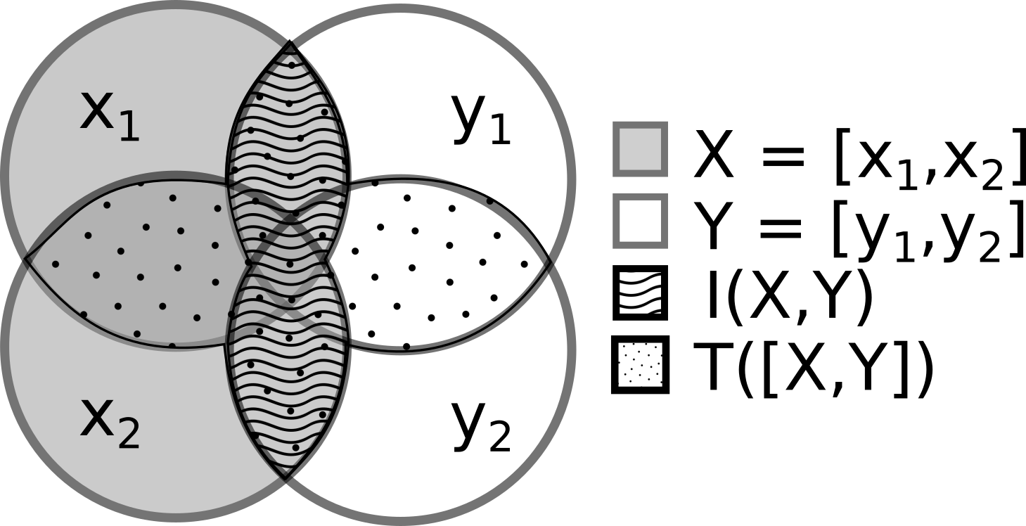
Mutual Information
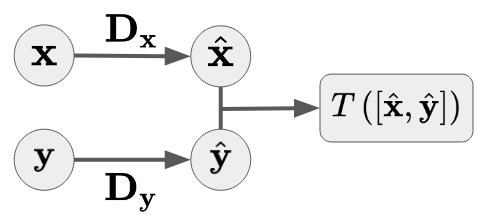
Given two random vectors $\mathbf{X}$ and $\mathbf{Y}$, we first Gaussianize each independently, then measure the total correlation of the joint:
$$I(\mathbf{X}, \mathbf{Y}) = T\!\left(\left[ \mathcal{G}_\theta(\mathbf{X}),\; \mathcal{G}_\phi(\mathbf{Y}) \right]\right)$$
KL-Divergence
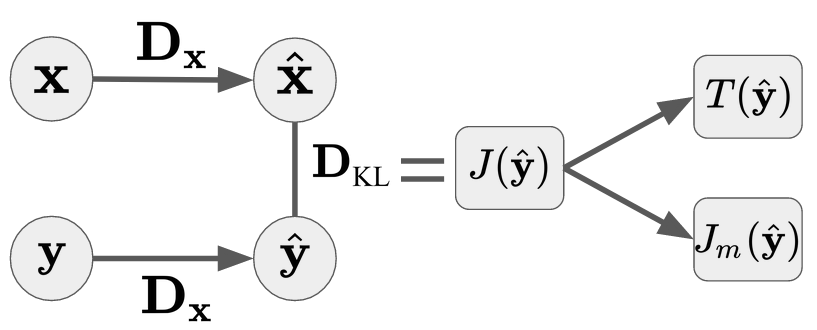
We estimate KL-divergence by applying the Gaussianization learned on $\mathbf{Y}$ to samples from $\mathbf{X}$:
$$D_\text{KL}\!\left[\mathbf{X} \| \mathbf{Y}\right] = J\!\left[\mathcal{G}_\theta(\hat{\mathbf{y}})\right]$$
See notebook 06 for the functional API and notebooks 09-11 for practical examples.
Summary
| Concept | Description |
|---|---|
| Gaussianization | Invertible transform mapping data to $\mathcal{N}(0, \mathbf{I})$ |
| Density Destructor | Destroys structure iteratively; enables exact likelihood via change of variables |
| Objective | Minimize total correlation (equivalently, maximize negentropy) |
| RBIG iteration | $\mathbf{x}^{(k+1)} = \mathbf{R}_{(k)} \cdot \mathbf{\Psi}_{(k)}(\mathbf{x}^{(k)})$ |
| IT measures | Entropy, MI, KLD estimated as by-products of the Gaussianization |
| API Class | Role |
|---|---|
MarginalGaussianize |
Marginal Gaussianization via empirical CDF + probit |
PCARotation |
Whitening PCA rotation |
RBIGLayer |
One RBIG layer = marginal + rotation |
AnnealedRBIG |
Full iterative model with convergence detection |