Information Theory Measures with RBIG¶

A key advantage of RBIG is that information-theoretic quantities fall out naturally from the Gaussianization process. This notebook demonstrates two approaches for estimating them, and compares both against analytical values on Gaussian data where ground truth is available.

Information Theory measures computable via RBIG.

Approach	How it works	Pros
Change-of-variables	Fit a full RBIG model, use the learned density	Single model, exact density
RBIG-way	Sum per-layer TC reductions	No Jacobian needed, more stable

Colab / fresh environment? Run the cell below to install rbig from GitHub. Skip if already installed.

In [1]:

!pip install "rbig[all] @ git+https://github.com/jejjohnson/rbig.git" -q

!pip install "rbig[all] @ git+https://github.com/jejjohnson/rbig.git" -q

In [2]:

import numpy as np
from scipy import stats

from rbig import (
    AnnealedRBIG,
    entropy_rbig,
    estimate_entropy,
    estimate_kld,
    estimate_mi,
    estimate_tc,
    kl_divergence_rbig,
    marginal_entropy,
    mutual_information_rbig,
    total_correlation_rbig,
)

import numpy as np from scipy import stats from rbig import ( AnnealedRBIG, entropy_rbig, estimate_entropy, estimate_kld, estimate_mi, estimate_tc, kl_divergence_rbig, marginal_entropy, mutual_information_rbig, total_correlation_rbig, )

/anaconda/lib/python3.13/site-packages/tqdm/auto.py:21: TqdmWarning: IProgress not found. Please update jupyter and ipywidgets. See https://ipywidgets.readthedocs.io/en/stable/user_install.html
  from .autonotebook import tqdm as notebook_tqdm

---

Shared Data Setup¶

We use correlated Gaussian data throughout so we can compare all estimates against closed-form analytical values.

Note: n_samples is kept small for fast execution; increase it (e.g. 10 000+) for closer agreement with analytical values.

In [3]:

seed = 42
rng = np.random.RandomState(seed)
n_samples = 1_000
d = 2  # dimensionality per block

# Joint covariance for [X, Y] with cross-correlations
C_full = np.eye(2 * d)
C_full[0, d] = C_full[d, 0] = 0.8  # x0 ↔ y0
C_full[1, d + 1] = C_full[d + 1, 1] = 0.5  # x1 ↔ y1

joint = rng.multivariate_normal(np.zeros(2 * d), C_full, size=n_samples)
X = joint[:, :d]
Y = joint[:, d:]
XY = joint

# Marginal covariances
CX = C_full[:d, :d]
CY = C_full[d:, d:]

# For KLD: shifted-mean distribution
mu_shift = np.array([0.5, 0.0])
X_shifted = rng.multivariate_normal(mu_shift, CX, size=n_samples)

# Common RBIG settings
rbig_kw = dict(n_layers=20, rotation="pca", patience=10, random_state=seed)

seed = 42 rng = np.random.RandomState(seed) n_samples = 1_000 d = 2 # dimensionality per block # Joint covariance for [X, Y] with cross-correlations C_full = np.eye(2 * d) C_full[0, d] = C_full[d, 0] = 0.8 # x0 ↔ y0 C_full[1, d + 1] = C_full[d + 1, 1] = 0.5 # x1 ↔ y1 joint = rng.multivariate_normal(np.zeros(2 * d), C_full, size=n_samples) X = joint[:, :d] Y = joint[:, d:] XY = joint # Marginal covariances CX = C_full[:d, :d] CY = C_full[d:, d:] # For KLD: shifted-mean distribution mu_shift = np.array([0.5, 0.0]) X_shifted = rng.multivariate_normal(mu_shift, CX, size=n_samples) # Common RBIG settings rbig_kw = dict(n_layers=20, rotation="pca", patience=10, random_state=seed)

---

1. Total Correlation¶

Total correlation measures the overall statistical dependence among all dimensions of a random vector — how far the joint distribution is from being fully independent:

$$\mathrm{TC}(X) = \sum_i H(X_i) - H(X) = D_\text{KL}\left[ p(\mathbf{x}) \| \prod_d p(x_d) \right]$$

TC is zero if and only if all dimensions are independent. In 2D, TC equals the mutual information.

Analytical¶

In [4]:

tc_true_X = 0.5 * (np.sum(np.log(np.diag(CX))) - np.log(np.linalg.det(CX)))
tc_true_XY = 0.5 * (np.sum(np.log(np.diag(C_full))) - np.log(np.linalg.det(C_full)))
print(f"TC(X)  analytical: {tc_true_X:.4f} nats")
print(f"TC(XY) analytical: {tc_true_XY:.4f} nats")

tc_true_X = 0.5 * (np.sum(np.log(np.diag(CX))) - np.log(np.linalg.det(CX))) tc_true_XY = 0.5 * (np.sum(np.log(np.diag(C_full))) - np.log(np.linalg.det(C_full))) print(f"TC(X) analytical: {tc_true_X:.4f} nats") print(f"TC(XY) analytical: {tc_true_XY:.4f} nats")

TC(X)  analytical: 0.0000 nats
TC(XY) analytical: 0.6547 nats

Change-of-variables (single-shot KDE + Gaussian joint)¶

In [5]:

tc_cov_X = total_correlation_rbig(X)
tc_cov_XY = total_correlation_rbig(XY)
print(f"TC(X)  change-of-vars: {tc_cov_X:.4f} nats")
print(f"TC(XY) change-of-vars: {tc_cov_XY:.4f} nats")

tc_cov_X = total_correlation_rbig(X) tc_cov_XY = total_correlation_rbig(XY) print(f"TC(X) change-of-vars: {tc_cov_X:.4f} nats") print(f"TC(XY) change-of-vars: {tc_cov_XY:.4f} nats")

TC(X)  change-of-vars: -0.0059 nats
TC(XY) change-of-vars: 0.6094 nats

RBIG-way (per-layer TC reduction)¶

In [6]:

tc_rbig_X = estimate_tc(X, **rbig_kw)
tc_rbig_XY = estimate_tc(XY, **rbig_kw)
print(f"TC(X)  RBIG-way: {tc_rbig_X:.4f} nats")
print(f"TC(XY) RBIG-way: {tc_rbig_XY:.4f} nats")

tc_rbig_X = estimate_tc(X, **rbig_kw) tc_rbig_XY = estimate_tc(XY, **rbig_kw) print(f"TC(X) RBIG-way: {tc_rbig_X:.4f} nats") print(f"TC(XY) RBIG-way: {tc_rbig_XY:.4f} nats")

TC(X)  RBIG-way: -0.0062 nats
TC(XY) RBIG-way: 0.6201 nats

---

2. Entropy¶

Entropy measures the uncertainty of a random variable — the expected information content:

$$H(X) = -\int p(x) \log p(x) \, dx$$

For Gaussian data: $H(X) = \frac{1}{2}\log\lvert 2\pi e\,\Sigma \rvert$

RBIG-way: $H(X) = \sum_d H(X_d) - \mathrm{TC}(X)$ — marginal entropies minus the RBIG-accumulated total correlation (no Jacobian needed).

Change-of-variables: $H(X) = -\mathbb{E}[\log p(x)]$ using the normalizing-flow density $\log p(x) = \log p_Z(f(x)) + \log\lvert\det J\rvert$.

Analytical¶

In [7]:

H_X_true = 0.5 * np.log(np.linalg.det(2 * np.pi * np.e * CX))
H_XY_true = 0.5 * np.log(np.linalg.det(2 * np.pi * np.e * C_full))
print(f"H(X)  analytical: {H_X_true:.4f} nats")
print(f"H(XY) analytical: {H_XY_true:.4f} nats")

H_X_true = 0.5 * np.log(np.linalg.det(2 * np.pi * np.e * CX)) H_XY_true = 0.5 * np.log(np.linalg.det(2 * np.pi * np.e * C_full)) print(f"H(X) analytical: {H_X_true:.4f} nats") print(f"H(XY) analytical: {H_XY_true:.4f} nats")

H(X)  analytical: 2.8379 nats
H(XY) analytical: 5.0211 nats

Change-of-variables¶

In [8]:

model_X = AnnealedRBIG(**rbig_kw).fit(X)
model_XY = AnnealedRBIG(**rbig_kw).fit(XY)

H_X_cov = model_X.entropy()
H_XY_cov = model_XY.entropy()
print(f"H(X)  change-of-vars: {H_X_cov:.4f} nats")
print(f"H(XY) change-of-vars: {H_XY_cov:.4f} nats")

model_X = AnnealedRBIG(**rbig_kw).fit(X) model_XY = AnnealedRBIG(**rbig_kw).fit(XY) H_X_cov = model_X.entropy() H_XY_cov = model_XY.entropy() print(f"H(X) change-of-vars: {H_X_cov:.4f} nats") print(f"H(XY) change-of-vars: {H_XY_cov:.4f} nats")

H(X)  change-of-vars: 2.8450 nats
H(XY) change-of-vars: 4.7623 nats

RBIG-way¶

In [9]:

H_X_rbig = estimate_entropy(X, **rbig_kw)
H_XY_rbig = estimate_entropy(XY, **rbig_kw)
print(f"H(X)  RBIG-way: {H_X_rbig:.4f} nats")
print(f"H(XY) RBIG-way: {H_XY_rbig:.4f} nats")

H_X_rbig = estimate_entropy(X, **rbig_kw) H_XY_rbig = estimate_entropy(XY, **rbig_kw) print(f"H(X) RBIG-way: {H_X_rbig:.4f} nats") print(f"H(XY) RBIG-way: {H_XY_rbig:.4f} nats")

H(X)  RBIG-way: 2.8369 nats
H(XY) RBIG-way: 4.9964 nats

---

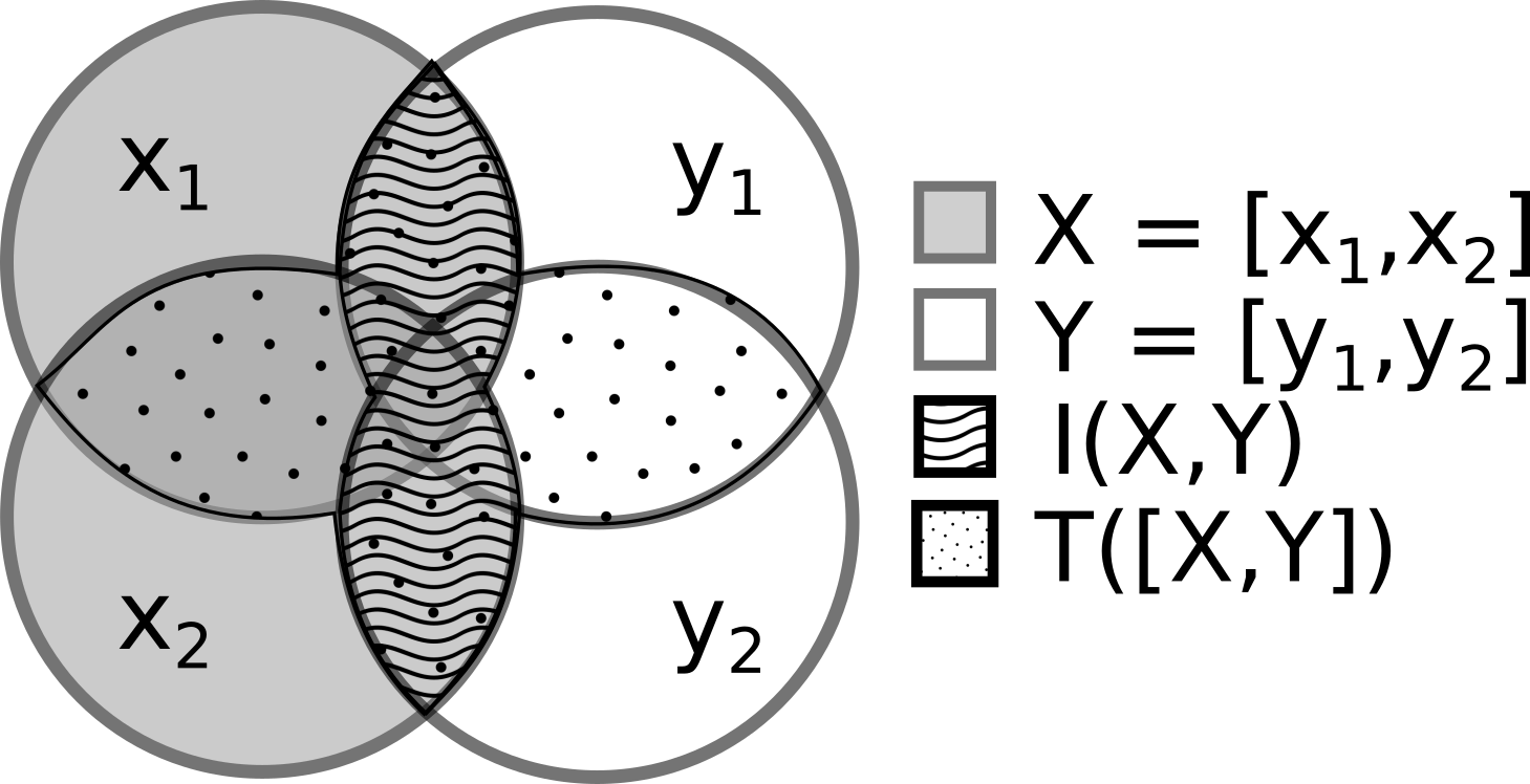
3. Mutual Information¶

Mutual information quantifies how much knowing $X$ tells you about $Y$ (and vice versa). It is zero if and only if $X$ and $Y$ are independent — unlike linear correlation, MI captures all forms of dependence:

$$\mathrm{MI}(X;Y) = H(X) + H(Y) - H(X,Y)$$

RBIG-way: $\mathrm{MI}(X;Y) = \mathrm{TC}([G_X(X),\, G_Y(Y)])$ — Gaussianize each block independently, then measure the TC of the concatenation.

Analytical¶

In [10]:

H_Y_true = 0.5 * np.log(np.linalg.det(2 * np.pi * np.e * CY))
mi_true = H_X_true + H_Y_true - H_XY_true
print(f"MI(X;Y) analytical: {mi_true:.4f} nats")

H_Y_true = 0.5 * np.log(np.linalg.det(2 * np.pi * np.e * CY)) mi_true = H_X_true + H_Y_true - H_XY_true print(f"MI(X;Y) analytical: {mi_true:.4f} nats")

MI(X;Y) analytical: 0.6547 nats

Change-of-variables (3 separate RBIG models)¶

In [11]:

model_Y = AnnealedRBIG(**rbig_kw).fit(Y)
mi_cov = mutual_information_rbig(model_X, model_Y, model_XY)
print(f"MI(X;Y) change-of-vars: {mi_cov:.4f} nats")

model_Y = AnnealedRBIG(**rbig_kw).fit(Y) mi_cov = mutual_information_rbig(model_X, model_Y, model_XY) print(f"MI(X;Y) change-of-vars: {mi_cov:.4f} nats")

MI(X;Y) change-of-vars: 0.8795 nats

RBIG-way (2 models + TC measurement)¶

In [12]:

mi_rbig = estimate_mi(X, Y, **rbig_kw)
print(f"MI(X;Y) RBIG-way: {mi_rbig:.4f} nats")

mi_rbig = estimate_mi(X, Y, **rbig_kw) print(f"MI(X;Y) RBIG-way: {mi_rbig:.4f} nats")

MI(X;Y) RBIG-way: 0.6325 nats

---

4. KL Divergence¶

KL-divergence measures how one probability distribution $P$ differs from a reference distribution $Q$. It is asymmetric and always non-negative:

$$\mathrm{KL}(P \| Q) = \int p(x) \log\frac{p(x)}{q(x)}\,dx$$

RBIG-way: $\mathrm{KL}(P_X \| P_Y) = \sum_d D(Z_d \| \mathcal{N}(0,1)) + \mathrm{TC}(Z)$ where $Z = G_Y(X)$ — apply Y's Gaussianization to X's samples, then measure per-marginal KL to standard Gaussian plus the TC of Z.

Change-of-variables: Uses cross-scoring of P's density model on Q's samples.

Analytical¶

Same covariance, shifted mean: $$\mathrm{KL}(\mathcal{N}(\mu, \Sigma) \| \mathcal{N}(0, \Sigma)) = \tfrac{1}{2}\mu^\top \Sigma^{-1} \mu$$

In [13]:

kld_true = 0.5 * mu_shift @ np.linalg.solve(CX, mu_shift)
print(f"KLD analytical: {kld_true:.4f} nats")

kld_true = 0.5 * mu_shift @ np.linalg.solve(CX, mu_shift) print(f"KLD analytical: {kld_true:.4f} nats")

KLD analytical: 0.1250 nats

Change-of-variables¶

In [14]:

# Fit model on the reference (unshifted) distribution
model_ref = AnnealedRBIG(**rbig_kw).fit(X)
kld_cov = kl_divergence_rbig(model_ref, X_shifted)
print(f"KLD change-of-vars: {kld_cov:.4f} nats")

# Fit model on the reference (unshifted) distribution model_ref = AnnealedRBIG(**rbig_kw).fit(X) kld_cov = kl_divergence_rbig(model_ref, X_shifted) print(f"KLD change-of-vars: {kld_cov:.4f} nats")

KLD change-of-vars: 0.4802 nats

RBIG-way¶

In [15]:

kld_rbig = estimate_kld(X_shifted, X, **rbig_kw)
print(f"KLD RBIG-way: {kld_rbig:.4f} nats")

kld_rbig = estimate_kld(X_shifted, X, **rbig_kw) print(f"KLD RBIG-way: {kld_rbig:.4f} nats")

KLD RBIG-way: 0.1123 nats

---

Comparison Table¶

All measures side-by-side: analytical ground truth vs. the two RBIG approaches.

In [16]:

print(f"{'Measure':<12} {'Analytical':>12} {'Change-of-Vars':>16} {'RBIG-way':>12}")
print("-" * 56)
print(f"{'TC(X)':12} {tc_true_X:12.4f} {tc_cov_X:16.4f} {tc_rbig_X:12.4f}")
print(f"{'TC(X,Y)':12} {tc_true_XY:12.4f} {tc_cov_XY:16.4f} {tc_rbig_XY:12.4f}")
print(f"{'H(X)':12} {H_X_true:12.4f} {H_X_cov:16.4f} {H_X_rbig:12.4f}")
print(f"{'H(X,Y)':12} {H_XY_true:12.4f} {H_XY_cov:16.4f} {H_XY_rbig:12.4f}")
print(f"{'MI(X;Y)':12} {mi_true:12.4f} {mi_cov:16.4f} {mi_rbig:12.4f}")
print(f"{'KLD':12} {kld_true:12.4f} {kld_cov:16.4f} {kld_rbig:12.4f}")

print(f"{'Measure':<12} {'Analytical':>12} {'Change-of-Vars':>16} {'RBIG-way':>12}") print("-" * 56) print(f"{'TC(X)':12} {tc_true_X:12.4f} {tc_cov_X:16.4f} {tc_rbig_X:12.4f}") print(f"{'TC(X,Y)':12} {tc_true_XY:12.4f} {tc_cov_XY:16.4f} {tc_rbig_XY:12.4f}") print(f"{'H(X)':12} {H_X_true:12.4f} {H_X_cov:16.4f} {H_X_rbig:12.4f}") print(f"{'H(X,Y)':12} {H_XY_true:12.4f} {H_XY_cov:16.4f} {H_XY_rbig:12.4f}") print(f"{'MI(X;Y)':12} {mi_true:12.4f} {mi_cov:16.4f} {mi_rbig:12.4f}") print(f"{'KLD':12} {kld_true:12.4f} {kld_cov:16.4f} {kld_rbig:12.4f}")

Measure        Analytical   Change-of-Vars     RBIG-way
--------------------------------------------------------
TC(X)              0.0000          -0.0059      -0.0062
TC(X,Y)            0.6547           0.6094       0.6201
H(X)               2.8379           2.8450       2.8369
H(X,Y)             5.0211           4.7623       4.9964
MI(X;Y)            0.6547           0.8795       0.6325
KLD                0.1250           0.4802       0.1123

---

See Also¶

• Measuring Dependence: 1D Variables — MI for detecting nonlinear dependence in 1D
• Measuring Dependence: 2D Variables — MI for multivariate dependence
• Information Theory with Synthetic Stock-Market Data — IT measures on financial data

References¶

• Nonlinear Extraction of "Independent Components" of elliptically symmetric densities using radial Gaussianization — Lyu & Simoncelli (2008) — PDF