Probability Density Function
The probability that a variate, , has the value .
Cumulative Distribution Function
The probability that a variate, , takes a value less than or equal to .
From a TPP perspective, this is known as the lifetime distribution.
Survival Function
The probability that a variate, , takes a value greater than . In other words, this gives the probability that an event will happen past a value , e.g., time.
From a TPP perspective, i.e., where , we have the following properties:
The survival function is non-increasing.
At , , i.e., the probability of surviving past time 0 is 1.
At , , i.e., as time goes to infinity, the survival curve goes to 0.
In theory, the survival function is smooth. However, in practice, we may observe events on a discrete scale. For example, on a time scale we may have days, weeks, or months.
Quantile Function
We can write this as the quantile function
We often use this function to calculate the frequency estimation like the AEP or the ARI.
Inverse Survival Function
This is the same as the quantile function given in equation (6) except we set the probability equal to the survival probability
Annual Exceedence Probability
The recurrence interval is a measure of how often an event is expected to occur based on the probability of exceeding a given stage streshold. This threshold is called the annual exceedance probability. To calculate this, we can express the return period (in years) as
where is the annual exceedence probability (AEP) and is the number of years Wang & Holmes, 2020. The AEP is has a domain between 0 and 1, , and the return period, , has a domain between 1 and infinity, . This can be limiting when we consider sub-annual probabilities which would be elements less than 1. In addition, it can be incorrect when there is some wrong interpolation between 100 and 1.
![A figure showing the return period [years] vs the probability of exceedance, R_a.](/research_journal_v2/build/rp-dd149235346706ac5fb022d32068ff40.png)
Figure 1:A figure showing the return period [years] vs the probability of exceedance, .
Derivation
This section is based off of Wang & Holmes, 2020Davison & Smith, 1990. Let be an indicator variable that indicates whether in , at least one event occurs or not
Then, is a Bernoulli distribution with the probabilities
Usage
In practice, we can use this to calculate the return level given any arbitrary CDF function
Once we solve this for the quantity in terms of .
After we simplify the expression, we get the following relationship
where is the quantile function, i.e., the inverse CDF function, and .
Average Recurrence Interval
The average recurrence interval (ARI) is the average time between events for a specified duration at a given location. This term is associated with partial duration series (PDS) or peak-over-thresholds (POTs). This is also known as the Mean Inter-Arrival Time or the Mean Recurrence Interval.
where is the mean inter-arrival time measured in Wang & Holmes, 2020.
![A figure showing the average recurrence interval [years] vs the probability of recurrence, R_p.](/research_journal_v2/build/ari-ecd8985a9da4027b880afbe4a102a057.png)
Figure 1:A figure showing the average recurrence interval [years] vs the probability of recurrence, .
Derivation
This section is based off of Wang & Holmes, 2020. We assume that we have a counting process, , which is a Poisson process with a rate of occurrence, . Then the probability that there is at least 1 event in the time interval, , is given as the survival function of the exponential distribution:
The mean inter-arrival time is given as
The probability of at least 1 event in the interval is given as
and the probability that there is at least 1 event within 1 unit time interval is given as
Note: we can extend this for distributions where we have multiple criteria. For example, in marked HPP, we could have a 2D Poisson process given over the domain
$$
$$
So essentially, we state that
So, the probability of no exceedances of over a 1-year period is given by the Poisson distribution
Usage
In practice, we can use this to calculate the return level given any arbitrary CDF function
Once we solve this for the quantity in terms of , we get the following relationship
where is the quantile function, i.e., the inverse CDF function, and .
AEP vs ARI
There are some equivalences of these two quantities. Namely, we can write this as:
Figure 3 showcases the AEP vs the probability of recurrence. We see that they are almost the same except for near the upper tail. Figure 4 demonstrates the relationship better. We see that the ARI has the domain between whereas the RP has the domain between . So, there is a relationship between the two quantities but they are not the same due to the differences in the domain.
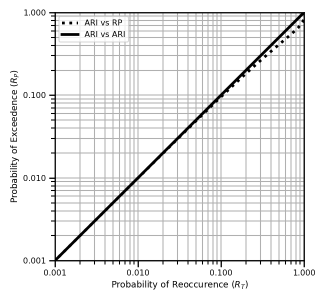
![A figure showing the average recurrence interval, T_p, [years] vs the return period, T_a[years].](/research_journal_v2/build/ari_vs_rp-bf9e9b76c997c24027ed95ea6ff3c935.png)
Hazard Function
The ratio of probability density function to the survival function, aka the conditional failure density function.
Counting Process
Survival Function
This is the probability that the time of death is later than some specified time, .
Event Density
This is the rate of death/failure events per unit time
Survival Event Density
Conditional Intensity Function
This is the instantaneous rate of a new arrival of new events at time, , given a history of past events, . This is also known as the hazard function.
We can rewrite this using th relationship of the survival function
We can also rewrite this using the relationship between the survival function and the cumulative hazard function
Cumulative Hazard Function
In general, there are four properties it needs to satisfy
This is achieved by always having a positive outcome within hazard function parameterization.
Probability Density Function
We can write the conditional probability density function in terms of the hazard and cumulative hazard function
We can also write it using the hazard function and the survival function
And lastly, we can write it in terms of the hazard function and the CDF function.
- Wang, C.-H., & Holmes, J. D. (2020). Exceedance rate, exceedance probability, and the duality of GEV and GPD for extreme hazard analysis. Natural Hazards, 102(3), 1305–1321. 10.1007/s11069-020-03968-z
- Davison, A. C., & Smith, R. L. (1990). Models for Exceedances Over High Thresholds. Journal of the Royal Statistical Society Series B: Statistical Methodology, 52(3), 393–425. 10.1111/j.2517-6161.1990.tb01796.x