Generalized Extreme Value Distribution
This is a location-scale family distribution.
Parameters ¶ Location : μ ∈ R Scale : σ ∈ R + Shape : κ ∈ R \begin{aligned}
\text{Location}: && &&
\boldsymbol{\mu} &\in \mathbb{R} \\
\text{Scale}: && &&
\boldsymbol{\sigma} &\in \mathbb{R}^+ \\
\text{Shape}: && &&
\boldsymbol{\kappa} &\in \mathbb{R} \\
\end{aligned} Location : Scale : Shape : μ σ κ ∈ R ∈ R + ∈ R Probability Density Function ¶ This is denoted as the probability that our rv Y Y Y
p ( Y = y ) : = f ( y ; θ ) p(Y=y) := f(y;\boldsymbol{\theta}) p ( Y = y ) := f ( y ; θ ) We can define the probability density function
f ( y ; θ ) = 1 σ t ( y ; θ ) κ + 1 e − t ( y ; θ ) \boldsymbol{f}(y;\boldsymbol{\theta}) =
\frac{1}{\sigma}t\left(y;\boldsymbol{\theta}\right)^{\kappa+1}e^{-t\left(y;\boldsymbol{\theta}\right)} f ( y ; θ ) = σ 1 t ( y ; θ ) κ + 1 e − t ( y ; θ ) where the function t ( y ; θ ) t(y;\boldsymbol{\theta}) t ( y ; θ )
t ( y ; θ ) = { [ 1 + κ ( y − μ σ ) ] + − 1 / κ , κ ≠ 0 exp ( − y − μ σ ) , κ = 0 \boldsymbol{t}(y;\boldsymbol{\theta}) =
\begin{cases}
\left[ 1 + \kappa \left( \frac{y-\mu}{\sigma} \right)\right]_+^{-1/\kappa}, && \kappa\neq 0 \\
\exp\left(-\frac{y-\mu}{\sigma}\right), && \kappa=0
\end{cases} t ( y ; θ ) = { [ 1 + κ ( σ y − μ ) ] + − 1/ κ , exp ( − σ y − μ ) , κ = 0 κ = 0 From
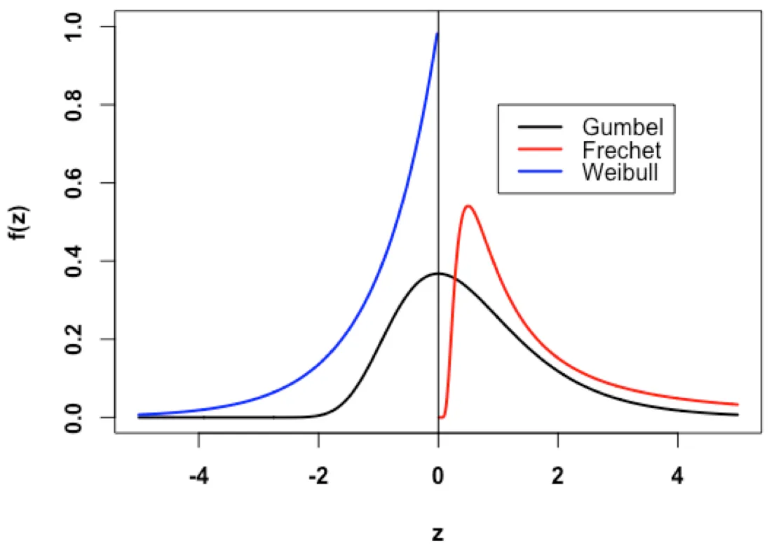
Figure 1: Some different distribution types for the GEVD - Source - Medium Article
Cumulative Distribution Function ¶ This is denoted as the probability that our rv Y Y Y y y y
p ( Y ≤ y ) : = F ( y ; θ ) p(Y\leq y) := F(y;\boldsymbol{\theta}) p ( Y ≤ y ) := F ( y ; θ ) We can define the cumulative density function
F ( y ; θ ) = exp [ − t ( y ; θ ) ] \boldsymbol{F}(y;\boldsymbol{\theta}) =
\exp
\left[ -\boldsymbol{t}(y;\boldsymbol{\theta}) \right] F ( y ; θ ) = exp [ − t ( y ; θ ) ] where the function t ( y ; θ ) t(y;\boldsymbol{\theta}) t ( y ; θ ) (4)
Survival Function ¶ This is the probability that our value of interest y y y
p ( Y > y ) : = S ( y ) p(Y>y) := \boldsymbol{S}(y) p ( Y > y ) := S ( y ) We denote this as:
S G E V D ( y ; θ ) = 1 − F ( y ; θ ) \boldsymbol{S}_{GEVD}(y;\boldsymbol{\theta}) = 1 - \boldsymbol{F}(y;\boldsymbol{\theta}) S GE V D ( y ; θ ) = 1 − F ( y ; θ ) We can plug in the CDF function into this equation
S ( y ; θ ) = 1 − exp [ − t ( y ; θ ) ] \boldsymbol{S}(y;\boldsymbol{\theta}) =
1 - \exp
\left[ -\boldsymbol{t}(y;\boldsymbol{\theta}) \right] S ( y ; θ ) = 1 − exp [ − t ( y ; θ ) ] where the function t ( y ; θ ) t(y;\boldsymbol{\theta}) t ( y ; θ ) (4)
Quantile Function ¶ This is also known as the Point-Percentile-Function or the inverse CDF .
This function maps an input threshold, y 0 y_0 y 0 y y y Y Y Y y y y y p y_p y p
y p = F ( y ; θ ) y_p = \boldsymbol{F}(y;\boldsymbol{\theta}) y p = F ( y ; θ ) We can take the inverse of this function to see that it is the inverse CDF which we denote as the quantile function.
y p = F − 1 ( y p ; θ ) : = Q ( y p ; θ ) y_p = \boldsymbol{F}^{-1}(y_p;\boldsymbol{\theta}) := \boldsymbol{Q}(y_p;\boldsymbol{\theta}) y p = F − 1 ( y p ; θ ) := Q ( y p ; θ ) where y p ∈ [ 0 , 1 ] y_p\in[0,1] y p ∈ [ 0 , 1 ]
Q ( y p ) = { μ + σ κ [ ( − log y p ) − κ − 1 ] κ ≠ 0 μ − σ log ( − log y p ) κ = 0 \boldsymbol{Q}(y_p) =
\begin{cases}
\mu + \frac{\sigma}{\kappa }\left[(- \log y_p)^{-\kappa} - 1 \right] && \kappa\neq 0 \\
\mu - \sigma\log(- \log y_p ) && \kappa=0
\end{cases} Q ( y p ) = { μ + κ σ [ ( − log y p ) − κ − 1 ] μ − σ log ( − log y p ) κ = 0 κ = 0
F ( y ; θ ) : = y p = exp [ − t ( y ; θ ) ] \boldsymbol{F}(y;\boldsymbol{\theta}) := y_p = \exp\left[-t(y;\boldsymbol{\theta})\right] F ( y ; θ ) := y p = exp [ − t ( y ; θ ) ] So let’s rearrange the terms within the equation
y p = exp [ − ( 1 + κ z ) − 1 / κ ] log y p = − ( 1 + κ z ) − 1 / κ − 1 κ log [ 1 + κ z ] = log ( − log y p ) log [ 1 + κ z ] = − κ log ( − log y p ) 1 + κ z = ( − log y p ) − κ κ z = ( − log y p ) − κ − 1 z = 1 κ [ ( − log y p ) − κ − 1 ] \begin{aligned}
y_p &= \exp\left[-(1 + \kappa z)^{-1/\kappa}\right] \\
\log y_p &=
-(1 + \kappa z)^{-1/\kappa}\\
-\frac{1}{\kappa}\log[1 + \kappa z] &=
\log \left( -\log y_p \right) \\
\log [1 + \kappa z] &=
-\kappa \log \left( -\log y_p\right) \\
1 + \kappa z &= (-\log y_p)^{-\kappa} \\
\kappa z &= (- \log y_p)^{-\kappa} - 1\\
z &= \frac{1}{\kappa}
\left[(- \log y_p)^{-\kappa} - 1 \right]
\end{aligned} y p log y p − κ 1 log [ 1 + κ z ] log [ 1 + κ z ] 1 + κ z κ z z = exp [ − ( 1 + κ z ) − 1/ κ ] = − ( 1 + κ z ) − 1/ κ = log ( − log y p ) = − κ log ( − log y p ) = ( − log y p ) − κ = ( − log y p ) − κ − 1 = κ 1 [ ( − log y p ) − κ − 1 ] Finally, we plug in our normalized variable
y = μ + σ κ [ ( − log y p ) − κ − 1 ] y = \mu + \frac{\sigma}{\kappa }\left[(- \log y_p)^{-\kappa} - 1 \right] y = μ + κ σ [ ( − log y p ) − κ − 1 ]
F ( y ; θ ) : = y p = exp ( − t ( y ; θ ) ) \boldsymbol{F}(y;\boldsymbol{\theta}) := y_p = \exp (-\boldsymbol{t}(y;\boldsymbol{\theta})) F ( y ; θ ) := y p = exp ( − t ( y ; θ )) So let’s rearrange the terms within the equation
y p = exp ( − exp ( − z ) ) log y p = − exp ( − z ) exp ( − z ) = − log y p z = − log ( − log y p ) \begin{aligned}
y_p &= \exp (-\exp(-z)) \\
\log y_p &= -\exp(-z)\\
\exp(-z) &= -\log y_p\\
z &=
-\log(- \log y_p )
\end{aligned} y p log y p exp ( − z ) z = exp ( − exp ( − z )) = − exp ( − z ) = − log y p = − log ( − log y p ) Finally, we plug in our normalized variable
y = μ − σ log ( − log y p ) y = \mu - \sigma\log(- \log y_p ) y = μ − σ log ( − log y p )
We can create an likelihood function for the quantile function where κ ≠ 0 \kappa\neq 0 κ = 0
# function for kappa > 0
def quantile(, loc, scale, shape):
    level = loc - scale / shape * (1 - (- log(1 - p)) ** (- shape))
    return level
We can also create a quantile function where κ = 0 \kappa=0 κ = 0
# function for kappa = 0
def quantile(p, loc, scale):
    level = loc - scale * log(- log())
    return level
Return Period ¶ We can calculate the RP using equation (8) GEVD (equation (6)
1 / T R = 1 − F ( y ; θ ) 1/T_R =
1 - \boldsymbol{F}(y;\boldsymbol{\theta}) 1/ T R = 1 − F ( y ; θ ) To make things simpler, we can simply use the quantile function in equation (12)
y p = 1 − 1 / T R y_p = 1 - 1 / T_R y p = 1 − 1/ T R However, if we expand this out, we get
y = { μ + σ κ { [ log ( 1 − 1 / T R ) ] κ − 1 } κ ≠ 0 μ − σ log [ − log ( 1 − 1 / T R ) ] κ = 0 y =
\begin{cases}
\mu + \frac{\sigma}{\kappa}\left\{\left[\log\left(1-1/T_R\right)\right]^{\kappa}-1\right\} && \kappa\neq 0 \\
\mu - \sigma \log \left[ - \log \left(1 - 1/T_R \right) \right] && \kappa=0
\end{cases} y = { μ + κ σ { [ log ( 1 − 1/ T R ) ] κ − 1 } μ − σ log [ − log ( 1 − 1/ T R ) ] κ = 0 κ = 0
In general, we can expand the RHS of the equation to include the CDF
1 − 1 / T R = exp ( − t ( y ; θ ) ) 1 - 1/T_R = \exp \left( -t(y;\boldsymbol{\theta}) \right) 1 − 1/ T R = exp ( − t ( y ; θ ) ) and we can reduce this to be:
− log ( 1 − 1 / T R ) = t ( y ; θ ) -\log\left(1-1/T_R\right) = t(y;\boldsymbol{\theta}) − log ( 1 − 1/ T R ) = t ( y ; θ ) Finally, we can plug in the κ ≠ 0 \kappa \neq 0 κ = 0
− log ( 1 − 1 / T R ) = [ 1 + κ z ] + − 1 / κ log [ − log ( 1 − 1 / T R ) ] = − ( 1 / κ ) log [ 1 + κ z ] log ( 1 + κ z ) = − κ log [ − log ( 1 − 1 / T R ) ] 1 + κ z = [ − log ( 1 − 1 / T R ) ] − κ κ z = [ log ( 1 − 1 / T R ) ] κ − 1 z = 1 κ { [ log ( 1 − 1 / T R ) ] κ − 1 } \begin{aligned}
-\log\left(1-1/T_R\right) &= [1 + \kappa z]_+^{-1/\kappa} \\
\log\left[-\log\left(1-1/T_R\right)\right]&= -(1/\kappa)\log[1 + \kappa z] \\
\log(1+\kappa z) &= -\kappa\log\left[-\log\left(1-1/T_R\right)\right] \\
1+\kappa z &=\left[-\log\left(1-1/T_R\right)\right]^{-\kappa} \\
\kappa z &= \left[\log\left(1-1/T_R\right)\right]^{\kappa}-1\\
z &= \frac{1}{\kappa}\left\{\left[\log\left(1-1/T_R\right)\right]^{\kappa}-1\right\} \\
\end{aligned} − log ( 1 − 1/ T R ) log [ − log ( 1 − 1/ T R ) ] log ( 1 + κ z ) 1 + κ z κ z z = [ 1 + κ z ] + − 1/ κ = − ( 1/ κ ) log [ 1 + κ z ] = − κ log [ − log ( 1 − 1/ T R ) ] = [ − log ( 1 − 1/ T R ) ] − κ = [ log ( 1 − 1/ T R ) ] κ − 1 = κ 1 { [ log ( 1 − 1/ T R ) ] κ − 1 } Now, we can plug in the normalization factor
y = μ + σ κ { [ log ( 1 − 1 / T R ) ] κ − 1 } y = \mu + \frac{\sigma}{\kappa}\left\{\left[\log\left(1-1/T_R\right)\right]^{\kappa}-1\right\} y = μ + κ σ { [ log ( 1 − 1/ T R ) ] κ − 1 } We can do the same thing for κ = 0 \kappa = 0 κ = 0
− log ( 1 − 1 / T R ) = exp ( − z ) log ( − log ( 1 − 1 / T R ) ) = − z z = − log ( − log ( 1 − 1 / T R ) ) \begin{aligned}
-\log (1 - 1/T_R) &= \exp(-z) \\
\log \left(-\log(1 - 1/T_R)\right) &= - z \\
z &= - \log \left(-\log(1 - 1/T_R)\right) \\
\end{aligned} − log ( 1 − 1/ T R ) log ( − log ( 1 − 1/ T R ) ) z = exp ( − z ) = − z = − log ( − log ( 1 − 1/ T R ) ) Now, we can plug in the normalization factor
y = μ − σ log [ − log ( 1 − 1 / T R ) ] y = \mu - \sigma \log \left[ - \log \left(1 - 1/T_R \right) \right] y = μ − σ log [ − log ( 1 − 1/ T R ) ] Average Recurrence Interval ¶ We can calculate the ARI using equation (14) GEVD (equation (6)
1 − exp ( − 1 / T ˉ ) = 1 − F ( y ; θ ) 1 - \exp\left(-1/\bar{T}\right) =
1 - \boldsymbol{F}(y;\boldsymbol{\theta}) 1 − exp ( − 1/ T ˉ ) = 1 − F ( y ; θ ) To make things simpler, we can simply use the quantile function in equation (12)
y p = exp ( − 1 / T ˉ ) y_p = \exp\left(-1/\bar{T}\right) y p = exp ( − 1/ T ˉ ) However, if we expand this out and simplify, we get
y = { μ + σ κ ( T ˉ κ − 1 ) κ ≠ 0 μ + σ log T ˉ κ = 0 y =
\begin{cases}
\mu + \frac{\sigma}{\kappa}\left( \bar{T}^{\kappa}-1\right) && \kappa\neq 0 \\
\mu + \sigma\log \bar{T} && \kappa=0
\end{cases} y = { μ + κ σ ( T ˉ κ − 1 ) μ + σ log T ˉ κ = 0 κ = 0
In general, we can expand the RHS of the equation to include the CDF
exp ( − 1 / T ˉ ) = exp ( − t ( y ; θ ) ) \exp(-1/\bar{T}) = \exp \left( -t(y;\boldsymbol{\theta}) \right) exp ( − 1/ T ˉ ) = exp ( − t ( y ; θ ) ) and we can reduce this to be:
1 / T ˉ = t ( y ; θ ) 1/\bar{T} = t(y;\boldsymbol{\theta}) 1/ T ˉ = t ( y ; θ ) Finally, we can plug in the κ ≠ 0 \kappa \neq 0 κ = 0
T ˉ = [ 1 + κ z ] + 1 / κ κ log T ˉ = log [ 1 + κ z ] 1 + κ z = T ˉ κ z = 1 κ ( T ˉ κ − 1 ) \begin{aligned}
\bar{T} &= [1 + \kappa z]_+^{1/\kappa} \\
\kappa \log \bar{T} &= \log [ 1 + \kappa z] \\
1 + \kappa z &= \bar{T}^{\kappa} \\
z &= \frac{1}{\kappa}\left( \bar{T}^{\kappa}-1\right) \\
\end{aligned} T ˉ κ log T ˉ 1 + κ z z = [ 1 + κ z ] + 1/ κ = log [ 1 + κ z ] = T ˉ κ = κ 1 ( T ˉ κ − 1 ) Now, we can plug in the normalization factor
y = μ + σ κ ( T ˉ κ − 1 ) y = \mu + \frac{\sigma}{\kappa}\left( \bar{T}^{\kappa}-1\right) y = μ + κ σ ( T ˉ κ − 1 ) We can do the same thing for κ = 0 \kappa = 0 κ = 0
1 / T ˉ = exp ( − z ) z = log T ˉ \begin{aligned}
1/\bar{T} &= \exp(-z) \\
z &= \log \bar{T}
\end{aligned} 1/ T ˉ z = exp ( − z ) = log T ˉ Now, we can plug in the normalization factor
y = μ + σ log T ˉ y = \mu + \sigma\log \bar{T} y = μ + σ log T ˉ Joint Distribution ¶ We can write the likelihood that the observations, y y y GEVD distribution.
So, given some observations, D = { y n } n = 1 N \mathcal{D}=\{y_n\}_{n=1}^{N} D = { y n } n = 1 N GEVD distribution, we can write the joint distribution decomposition as
p ( y 1 : N ; θ ) = p ( θ ) ∏ n = 1 N p ( y n ∣ θ ) p(y_{1:N};\boldsymbol{\theta}) =
p(\boldsymbol{\theta})
\prod_{n=1}^N
p(y_n|\boldsymbol{\theta}) p ( y 1 : N ; θ ) = p ( θ ) n = 1 ∏ N p ( y n ∣ θ ) This implies that the global prior parameters come from some distribution
θ ∼ p ( θ ) \boldsymbol{\theta} \sim p(\boldsymbol{\theta}) θ ∼ p ( θ ) and that these parameters get passed through our data likelihood term
y n ∼ p ( y ∣ θ ) y_n \sim p(y|\boldsymbol{\theta}) y n ∼ p ( y ∣ θ ) Log Probability ¶ Recall the PDF for our iid samples is
p ( y 1 : N ∣ θ ) = ∏ n = 1 N 1 σ t ( y n ; θ ) κ + 1 e − t ( y n ; θ ) p(y_{1:N}|\boldsymbol{\theta}) = \prod_{n=1}^N\frac{1}{\sigma}t\left(y_n;\boldsymbol{\theta}\right)^{\kappa+1}e^{-t\left(y_n;\boldsymbol{\theta}\right)} p ( y 1 : N ∣ θ ) = n = 1 ∏ N σ 1 t ( y n ; θ ) κ + 1 e − t ( y n ; θ ) where t ( y n ; θ ) t(y_n;\boldsymbol{\theta}) t ( y n ; θ ) (4)
log p ( y 1 : N ∣ θ ) = ∑ n = 1 N log p ( y n ∣ θ ) \log p(\boldsymbol{y}_{1:N}|\boldsymbol{\theta}) = \sum_{n=1}^N \log p(y_n|\boldsymbol{\theta}) log p ( y 1 : N ∣ θ ) = n = 1 ∑ N log p ( y n ∣ θ ) which we can expand as
∑ n = 1 N log p ( y n ; θ ) = − N log σ − ( 1 + 1 / κ ) ∑ n = 1 N log t ( y n ; θ ) − ∑ n = 1 N t ( y n ; θ ) \sum_{n=1}^N\log p(y_n;\boldsymbol{\theta}) =
-N \log \sigma -
(1+1/\kappa)\sum_{n=1}^N
\log t\left(y_n;\boldsymbol{\theta}\right) -
\sum_{n=1}^N t\left(y_n;\boldsymbol{\theta}\right) n = 1 ∑ N log p ( y n ; θ ) = − N log σ − ( 1 + 1/ κ ) n = 1 ∑ N log t ( y n ; θ ) − n = 1 ∑ N t ( y n ; θ ) which reduces to
log p ( y 1 : N ∣ θ ) = − N log σ − ( 1 + 1 / κ ) ∑ n = 1 N log [ 1 + κ z n ] + − ∑ n = 1 N [ 1 + κ z n ] + − 1 / κ \log p(\boldsymbol{y}_{1:N}|\boldsymbol{\theta}) =
- N \log \sigma -
(1+1/\kappa)\sum_{n=1}^N
\log \left[ 1 + \kappa z_n\right]_+
-
\sum_{n=1}^N
\left[ 1 + \kappa z_n\right]_+^{-1/\kappa} log p ( y 1 : N ∣ θ ) = − N log σ − ( 1 + 1/ κ ) n = 1 ∑ N log [ 1 + κ z n ] + − n = 1 ∑ N [ 1 + κ z n ] + − 1/ κ
We can create an likelihood function for this.
def gev_logpdf(x, location, scale, shape):
# calculate location scale: z=(y−μ)/σ
z = (x - mu) / sigma
# calculate t(z) = 1+κz
t = 1.0 + shape * z
# grab max value
t = np.max(t, 0)
# term 1: −log σ
t1 = - np.log(sigma)
# term 2: − (1+κz) ** −1/κ
t2 = - np.power(t, -1.0 / xi)
# term 3: - (1+1/κ)log(1+κz)
t3 = - (1.0 / xi + 1.0) * np.log(t)
return t1 + t2 + t3Instead of actually calculating the full scheme, we can simply apply this
y: Array["T"] = ...
params: PyTree = ...
# apply vectorized operation
nll: Array["T"] = vectorize(gev_logpdf, y, params)
# take the sume
nll: Scalar = sum(nll)
We are interested in calculating the log probability function
log p ( y 1 : N ∣ θ ) = ∑ n = 1 N log p ( y n ∣ θ ) \log p(\boldsymbol{y}_{1:N}|\boldsymbol{\theta}) = \sum_{n=1}^N \log p(y_n|\boldsymbol{\theta}) log p ( y 1 : N ∣ θ ) = n = 1 ∑ N log p ( y n ∣ θ ) Let’s consider only a single input, y n y_n y n t ( y n ; θ ) \boldsymbol{t}(y_n;\boldsymbol{\theta}) t ( y n ; θ )
p ( y n ∣ θ ) = 1 σ t ( y n ; θ ) κ + 1 e − t ( y n ; θ ) p(y_n|\boldsymbol{\theta}) = \frac{1}{\sigma}t\left(y_n;\boldsymbol{\theta}\right)^{\kappa+1}e^{-t\left(y_n;\boldsymbol{\theta}\right)} p ( y n ∣ θ ) = σ 1 t ( y n ; θ ) κ + 1 e − t ( y n ; θ ) Now, we apply the log function
log p ( y n ∣ θ ) = log ( 1 σ t ( y n ; θ ) κ + 1 e − t ( y n ; θ ) ) \log p(y_n|\boldsymbol{\theta}) = \log
\left(\frac{1}{\sigma}t\left(y_n;\boldsymbol{\theta}\right)^{\kappa+1}e^{-t\left(y_n;\boldsymbol{\theta}\right)}\right) log p ( y n ∣ θ ) = log ( σ 1 t ( y n ; θ ) κ + 1 e − t ( y n ; θ ) ) We can separate each of the terms
log p ( y n ∣ θ ) = log ( 1 σ ) + log ( t ( y n ; θ ) κ + 1 ) + log ( e − t ( y n ; θ ) ) \log p(y_n|\boldsymbol{\theta}) = \log
\left(\frac{1}{\sigma}\right) +
\log\left(t\left(y_n;\boldsymbol{\theta}\right)^{\kappa+1}\right) +
\log \left(e^{-t\left(y_n;\boldsymbol{\theta}\right)}\right) log p ( y n ∣ θ ) = log ( σ 1 ) + log ( t ( y n ; θ ) κ + 1 ) + log ( e − t ( y n ; θ ) ) Now we can do some log rules to simplify the terms
log p ( y n ∣ θ ) = − log σ + ( κ + 1 ) log t ( y n ; θ ) − t ( y n ; θ ) \log p(y_n|\boldsymbol{\theta}) =
-\log \sigma +
(\kappa+1) \log t\left(y_n;\boldsymbol{\theta}\right)
- t\left(y_n;\boldsymbol{\theta}\right) log p ( y n ∣ θ ) = − log σ + ( κ + 1 ) log t ( y n ; θ ) − t ( y n ; θ ) We can plug in the t ( y ; θ ) \boldsymbol{t}(y;\boldsymbol{\theta}) t ( y ; θ ) z = y − μ σ z=\frac{y-\mu}{\sigma} z = σ y − μ
log p ( y n ∣ θ ) = − log σ + ( κ + 1 ) log [ 1 + κ z ] + − 1 / κ − [ 1 + κ z ] + − 1 / κ \log p(y_n|\boldsymbol{\theta}) =
-\log \sigma +
(\kappa+1) \log \left[ 1 + \kappa z\right]_+^{-1/\kappa}
- \left[ 1 + \kappa z\right]_+^{-1/\kappa} log p ( y n ∣ θ ) = − log σ + ( κ + 1 ) log [ 1 + κ z ] + − 1/ κ − [ 1 + κ z ] + − 1/ κ We can do some final simplification
log p ( y n ∣ θ ) = − log σ − ( 1 + 1 / κ ) log [ 1 + κ z n ] + − [ 1 + κ z n ] + − 1 / κ \log p(y_n|\boldsymbol{\theta}) =
-\log \sigma -
(1+1/\kappa)\log \left[ 1 + \kappa z_n\right]_+
- \left[ 1 + \kappa z_n\right]_+^{-1/\kappa} log p ( y n ∣ θ ) = − log σ − ( 1 + 1/ κ ) log [ 1 + κ z n ] + − [ 1 + κ z n ] + − 1/ κ Now, we can plug in the sum
log p ( y 1 : N ∣ θ ) = ∑ n = 1 N ( − log σ − ( 1 + 1 / κ ) log [ 1 + κ z n ] + − [ 1 + κ z n ] + − 1 / κ ) \log p(\boldsymbol{y}_{1:N}|\boldsymbol{\theta}) =
\sum_{n=1}^N
\left(
-\log \sigma -
(1+1/\kappa)\log \left[ 1 + \kappa z_n\right]_+
- \left[ 1 + \kappa z_n\right]_+^{-1/\kappa}
\right) log p ( y 1 : N ∣ θ ) = n = 1 ∑ N ( − log σ − ( 1 + 1/ κ ) log [ 1 + κ z n ] + − [ 1 + κ z n ] + − 1/ κ ) We can factor out the constant values
log p ( y 1 : N ∣ θ ) = − N log σ − ( 1 + 1 / κ ) ∑ n = 1 N log [ 1 + κ z n ] + − ∑ n = 1 N [ 1 + κ z n ] + − 1 / κ \log p(\boldsymbol{y}_{1:N}|\boldsymbol{\theta}) =
- N \log \sigma -
(1+1/\kappa)\sum_{n=1}^N
\log \left[ 1 + \kappa z_n\right]_+
-
\sum_{n=1}^N
\left[ 1 + \kappa z_n\right]_+^{-1/\kappa} log p ( y 1 : N ∣ θ ) = − N log σ − ( 1 + 1/ κ ) n = 1 ∑ N log [ 1 + κ z n ] + − n = 1 ∑ N [ 1 + κ z n ] + − 1/ κ Reparameterization ¶ In this instance, we are assuming that there is a threshold parameter, y 0 y_0 y 0
μ = μ y 0 + σ y 0 κ ( 1 − λ y 0 − κ ) σ = σ y 0 λ y 0 − κ κ ≠ 0 μ = μ y 0 + σ y 0 ln λ y 0 σ = σ y 0 λ y 0 − κ κ = 0 \begin{aligned}
\mu &= \mu_{y_0} + \frac{\sigma_{y_0}}{\kappa}\left(1 - \lambda_{y_0}^{-\kappa} \right) && &&
\sigma =\sigma_{y_0}\lambda_{y_0}^{-\kappa} && &&
\kappa\neq0 \\
\mu &= \mu_{y_0} + \sigma_{y_0}\ln\lambda_{y_0} && &&
\sigma =\sigma_{y_0}\lambda_{y_0}^{-\kappa} && &&
\kappa=0 \\
\end{aligned} μ μ = μ y 0 + κ σ y 0 ( 1 − λ y 0 − κ ) = μ y 0 + σ y 0 ln λ y 0 σ = σ y 0 λ y 0 − κ σ = σ y 0 λ y 0 − κ κ = 0 κ = 0 Rescaling ¶ δ h = h h ∗ \delta_h = \frac{h}{h^*} δ h = h ∗ h where h h h h ∗ h^* h ∗
μ ∗ = μ + 1 κ [ σ ∗ ( 1 − δ h − κ ) ] σ ∗ = σ δ h κ κ ∗ = κ \begin{aligned}
\mu^* &= \mu + \frac{1}{\kappa}\left[\sigma^*(1-\delta_h^{-\kappa}) \right] \\
\sigma^* &= \sigma\delta_h^{\kappa} \\
\kappa^* &= \kappa
\end{aligned} μ ∗ σ ∗ κ ∗ = μ + κ 1 [ σ ∗ ( 1 − δ h − κ ) ] = σ δ h κ = κ Literature Review ¶ Theory .
Leadbetter et al. (1983)
Applications .
García et al. (2023) GEVD .
GEVD .
Algorithms .
Moins et al. (2023) Koh et al. (2021) PP for the events and a GPD for the marks.
Leadbetter, M. R., Lindgren, G., & Rootzén, H. (1983). Extremes and Related Properties of Random Sequences and Processes. In Springer Series in Statistics . Springer New York. 10.1007/978-1-4612-5449-2 García, J. A., Acero, F. J., & Portero, J. (2023). A Bayesian hierarchical spatio-temporal model for extreme temperatures in Extremadura (Spain) simulated by a Regional Climate Model. Climate Dynamics , 61 (3–4), 1489–1503. 10.1007/s00382-022-06638-x Moins, T., Arbel, J., Girard, S., & Dutfoy, A. (2023). Reparameterization of extreme value framework for improved Bayesian workflow. Computational Statistics & Data Analysis , 187 , 107807. 10.1016/j.csda.2023.107807 Koh, J., Pimont, F., Dupuy, J.-L., & Opitz, T. (2021). Spatiotemporal wildfire modeling through point processes with moderate and extreme marks . arXiv. 10.48550/ARXIV.2105.08004