Block Maximum
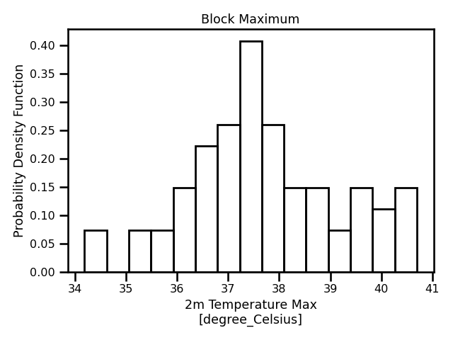
In these examples, we are applying the Block Maxima (BM) method on a yearly basis. So, our block size is of one year which leaves us 62 years in total for our time series. While this is not a lot of data, we see in Figure 5 that the distribution does match one of the classical GEVD distributions. In particular, the Fréchet distribution where the shape parameter, , is less than 0 (Figure 1).
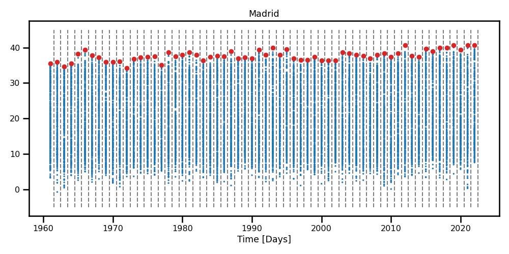
Figure 3: A scatter plot with boundaries for the maximum temperatures obtained using the yearly Block maxima method.
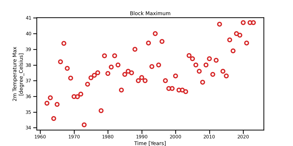
Figure 4: A scatter plot for the yearly maximum values obtained from the daily 2m max temperature for Madrid.
Figure 5: A histogram of all values obtained using the block maxima method.
In this figure, we have different representations for the block maximum method. We already see a trend line and perhaps a hint of cyclic behaviour. In our first experiments, we see will assume a unconditional distribution however we can see that this assumption is incorrect as we can clearly see from Figure 4.
Model Metrics
| Model | ELPD WAIC | ELPD WAIC SE | P WAIC |
|---|---|---|---|
| M0a | -157.11 | 4.68 | 0.01 |
| M0b | -96.57 | 3.74 | 1.46 |
| M0c | -97.18 | 3.87 | 1.30 |
| M1a | -96.57 | 3.74 | 1.46 |
| M1b | -96.43 | 3.68 | 1.86 |
| M2 | -97.19 | 5.06 | 1.85 |
| M3 | - 96.86 | 4.50 | 1.75 |
Stationary Models
Static Parameters
| Model | Location | Scale | Shape | 100-Year RP |
|---|---|---|---|---|
| M0a | 35.02 (0.05) | 4.24 (0.03) | -0.34 (0.00) | 44.81 (0.04) |
| M0b | 39.31 (0.21) | 1.47 (0.15) | -0.43 (0.08) | 42.22 (0.36) |
| M0c | 39.29 (0.19) | 1.41 (0.13) | -0.34 (0.01) | 42.54 (0.31) |
| M2 | 39.34 (0.17) | 1.25 (0.11) | -0.30 (0.01) | 42.44 (0.29) |
Non-Stationary Models
Static Parameters
| Model | Scale | Shape |
|---|---|---|
| M1 | 1.40 (0.14) | -0.35 (0.01) |
| M3 | 1.24 (0.11) | -0.29 (0.01) |
GMST Parameters
Location Parameters
| Model | Historical, 0.0 [C°] | Current, 1.0 [C°] | Future, 2.0 [C°] |
|---|---|---|---|
| M1 | 39.09 (0.27) | 39.69 (0.41) | 40.30 (0.94) |
| M3 | 38.75 (0.18) | 40.46 (0.20) | 42.22 (0.33) |
100-Year Return Level
| Model | Historical, 0.0 [C°] | Current, 1.0 [C°] | Future, 2.0 [C°] |
|---|---|---|---|
| M1 | 42.27 (0.36) | 42.88 (0.46) | 43.50 (0.96) |
| M3 | 41.90 (0.29) | 43.61 (0.32) | 45.38 (0.43) |