Ensemble Kalman Filter from Scratch

This notebook builds an Ensemble Kalman Filter (EnKF) step by step, using gaussx ensemble primitives on the chaotic Lorenz-63 system.

What you’ll learn:

Computing empirical covariance as a structured LowRankUpdate operator with gaussx.ensemble_covariance
Computing cross-covariance between state and observation ensembles with gaussx.ensemble_cross_covariance
Numerically stable covariance updates with gaussx.joseph_update
Deriving process noise from a stationary covariance with gaussx.process_noise_covariance

Background¶

The Ensemble Kalman Filter (Evensen, 1994) is a Monte Carlo approximation to the Kalman filter designed for high-dimensional, nonlinear systems. Instead of propagating a mean and covariance matrix explicitly, it maintains an ensemble of $J$ particles $\{x^{(j)}\}_{j=1}^{J}$ that collectively represent the state distribution.

The key idea: at each step the forecast covariance is estimated empirically from the ensemble spread, so no linearization (tangent linear model) is needed. The update step then applies the standard Kalman gain formula using these empirical statistics.

EnKF algorithm sketch¶

Forecast: Propagate each particle through the (possibly nonlinear) dynamics $x^{(j)}_{t|t-1} = f(x^{(j)}_{t-1|t-1}) + q^{(j)}_t$ .

Analysis:

Compute ensemble covariance: $\hat{P} = \frac{1}{J}\sum_j (x^{(j)} - \bar{x})(x^{(j)} - \bar{x})^\top$
Compute cross-covariance between state and predicted observations: $C_{xy} = \frac{1}{J}\sum_j (x^{(j)} - \bar{x})(y^{(j)} - \bar{y})^\top$
Compute innovation covariance: $C_{yy} = \frac{1}{J}\sum_j (y^{(j)} - \bar{y})(y^{(j)} - \bar{y})^\top + R$
Kalman gain: $K = C_{xy} \, C_{yy}^{-1}$
Perturbed-observation update: $x^{(j)}_{t|t} = x^{(j)}_{t|t-1} + K(y_t + \epsilon^{(j)} - H x^{(j)}_{t|t-1})$

from __future__ import annotations

import warnings


warnings.filterwarnings("ignore", message=r".*IProgress.*")

import jax
import jax.numpy as jnp
import matplotlib.pyplot as plt

import gaussx


jax.config.update("jax_enable_x64", True)

Define the Lorenz-63 system¶

The Lorenz-63 system is a classic chaotic dynamical system:

\frac{dx}{dt} = \sigma(y - x)

((1))

\frac{dy}{dt} = x(\rho - z) - y

((2))

\frac{dz}{dt} = xy - \beta z

((3))

With the standard parameters $\sigma = 10$ , $\rho = 28$ , $\beta = 8/3$ , the system exhibits the famous butterfly attractor. We discretize with a 4th-order Runge-Kutta integrator.

# Lorenz-63 parameters
sigma_l = 10.0
rho = 28.0
beta = 8.0 / 3.0
dt = 0.01


def lorenz63(state):
    """Lorenz-63 right-hand side."""
    x, y, z = state[0], state[1], state[2]
    dx = sigma_l * (y - x)
    dy = x * (rho - z) - y
    dz = x * y - beta * z
    return jnp.array([dx, dy, dz])


def rk4_step(state, _dt=dt):
    """Single RK4 integration step."""
    k1 = lorenz63(state)
    k2 = lorenz63(state + 0.5 * _dt * k1)
    k3 = lorenz63(state + 0.5 * _dt * k2)
    k4 = lorenz63(state + _dt * k3)
    return state + (_dt / 6.0) * (k1 + 2 * k2 + 2 * k3 + k4)


# Quick sanity check: integrate a short trajectory
x_test = jnp.array([1.0, 1.0, 1.0])
x_test_next = rk4_step(x_test)
print("One RK4 step: ", x_test, " -> ", x_test_next)

One RK4 step:  [1. 1. 1.]  ->  [1.01256719 1.2599178  0.98489097]

Generate the true trajectory and observations¶

We observe only the $x$ and $y$ components of the Lorenz state with additive Gaussian noise. The $z$ component must be inferred.

T = 500  # number of time steps
obs_noise_std = 2.0

# Observation model: observe x and y only
H = jnp.array([[1.0, 0.0, 0.0], [0.0, 1.0, 0.0]])
R = obs_noise_std**2 * jnp.eye(2)

# True initial condition (on the attractor)
x_true_0 = jnp.array([1.508, -1.531, 25.46])

key = jax.random.PRNGKey(42)


def generate_truth(carry, key_t):
    """Propagate true state and generate noisy observation."""
    x_true = carry
    x_true_next = rk4_step(x_true)
    noise = obs_noise_std * jax.random.normal(key_t, shape=(2,))
    y_t = H @ x_true_next + noise
    return x_true_next, (x_true_next, y_t)


keys_truth = jax.random.split(key, T)
_, (true_states, observations) = jax.lax.scan(generate_truth, x_true_0, keys_truth)

times = jnp.arange(T) * dt
print("True trajectory shape:", true_states.shape)
print("Observations shape:", observations.shape)

True trajectory shape: (500, 3)
Observations shape: (500, 2)

Initialize the ensemble¶

We draw $J = 50$ particles from a Gaussian centered at the true initial state with moderate uncertainty. In practice the initial ensemble would come from a climatological prior.

J = 50  # ensemble size
d = 3  # state dimension

P0 = jnp.diag(jnp.array([2.0, 2.0, 2.0]))

key, subkey = jax.random.split(key)
L0 = jnp.linalg.cholesky(P0)
ensemble = x_true_0[None, :] + jax.random.normal(subkey, shape=(J, d)) @ L0.T

print("Initial ensemble shape:", ensemble.shape)
print("Ensemble mean:", jnp.mean(ensemble, axis=0))

Initial ensemble shape: (50, 3)
Ensemble mean: [ 1.80543028 -1.45576339 25.35649402]

Inspect the ensemble covariance operator¶

Before running the filter, let’s see what gaussx.ensemble_covariance returns. It produces a LowRankUpdate operator -- a structured representation of $\hat{P} = (1/J)\sum_j \delta_j \delta_j^\top$ where $\delta_j = x^{(j)} - \bar{x}$ . This is rank $\leq J$ and avoids materializing the full $d \times d$ matrix (crucial when $d$ is large).

P_ens = gaussx.ensemble_covariance(ensemble)
print("Type:", type(P_ens).__name__)
print("Materialized covariance:\n", P_ens.as_matrix())

# Compare with naive computation
mean_ens = jnp.mean(ensemble, axis=0)
devs = ensemble - mean_ens[None, :]
P_naive = (devs.T @ devs) / J
print("\nNaive covariance:\n", P_naive)
print("Max difference:", jnp.max(jnp.abs(P_ens.as_matrix() - P_naive)))

Type: LowRankUpdate

Materialized covariance:
 [[ 1.89403362  0.18874692 -0.22508983]
 [ 0.18874692  1.90614772 -0.60569166]
 [-0.22508983 -0.60569166  2.1204657 ]]

Naive covariance:
 [[ 1.89403362  0.18874692 -0.22508983]
 [ 0.18874692  1.90614772 -0.60569166]
 [-0.22508983 -0.60569166  2.1204657 ]]
Max difference: 8.881784197001252e-16

Run the Ensemble Kalman Filter¶

The main loop: forecast each particle through the nonlinear Lorenz dynamics, then perform the EnKF analysis update using gaussx ensemble primitives.

We add a small amount of process noise (additive inflation) to prevent ensemble collapse, a common practical technique.

process_noise_std = 0.1
Q_enkf = process_noise_std**2 * jnp.eye(d)


def enkf_step(carry, inputs):
    """Single EnKF forecast + analysis step."""
    ensemble_prev, _key_prev = carry
    y_obs, key_t = inputs

    k1, k2, k3 = jax.random.split(key_t, 3)

    # --- Forecast: propagate each particle through nonlinear dynamics ---
    ensemble_pred = jax.vmap(rk4_step)(ensemble_prev)

    # Add process noise (additive inflation)
    q_noise = process_noise_std * jax.random.normal(k1, shape=(J, d))
    ensemble_pred = ensemble_pred + q_noise

    # --- Analysis: compute ensemble statistics using gaussx ---

    # Predicted observation ensemble: y_j = H @ x_j
    obs_pred = ensemble_pred @ H.T  # (J, 2)

    # Cross-covariance C_xy between state and predicted observations
    C_xy = gaussx.ensemble_cross_covariance(ensemble_pred, obs_pred)  # (3, 2)

    # Innovation covariance C_yy + R
    C_yy_op = gaussx.ensemble_covariance(obs_pred)
    C_yy = C_yy_op.as_matrix() + R  # (2, 2)

    # Kalman gain K = C_xy @ inv(C_yy)
    K = C_xy @ jnp.linalg.inv(C_yy)  # (3, 2)

    # Perturbed-observation update
    obs_noise = obs_noise_std * jax.random.normal(k2, shape=(J, 2))
    innovations = y_obs[None, :] + obs_noise - obs_pred  # (J, 2)
    ensemble_upd = ensemble_pred + innovations @ K.T  # (J, 3)

    # Ensemble mean for diagnostics
    mean_upd = jnp.mean(ensemble_upd, axis=0)

    return (ensemble_upd, k3), (mean_upd, ensemble_upd)


# Prepare inputs
keys_enkf = jax.random.split(jax.random.PRNGKey(123), T)
inputs = (observations, keys_enkf)

# Run the filter
init_carry = (ensemble, jax.random.PRNGKey(0))
_, (enkf_means, enkf_ensembles) = jax.lax.scan(enkf_step, init_carry, inputs)

print("EnKF means shape:", enkf_means.shape)
print("EnKF ensembles shape:", enkf_ensembles.shape)

EnKF means shape: (500, 3)
EnKF ensembles shape: (500, 50, 3)

Joseph-form covariance update¶

The standard EnKF implicitly updates the covariance via the ensemble. For diagnostics or hybrid filters, one sometimes needs the explicit updated covariance. The Joseph form

P_{\text{upd}} = (I - KH)\,P_{\text{pred}}\,(I - KH)^\top + K R K^\top

((4))

is numerically more stable than the naive $(I - KH) P_{\text{pred}}$ formula. Let’s demonstrate gaussx.joseph_update on the final step.

# Use the final forecast ensemble to get P_pred
final_ensemble_pred = jax.vmap(rk4_step)(enkf_ensembles[-1])
P_pred_op = gaussx.ensemble_covariance(final_ensemble_pred)
P_pred = P_pred_op.as_matrix()

# Recompute the Kalman gain for this step
obs_pred_final = final_ensemble_pred @ H.T
C_xy_final = gaussx.ensemble_cross_covariance(final_ensemble_pred, obs_pred_final)
C_yy_final = gaussx.ensemble_covariance(obs_pred_final).as_matrix() + R
K_final = C_xy_final @ jnp.linalg.inv(C_yy_final)

# Joseph-form update
P_upd_joseph = gaussx.joseph_update(P_pred, K_final, H, R)

# Compare with naive formula
I_KH = jnp.eye(d) - K_final @ H
P_upd_naive = I_KH @ P_pred

print("Joseph-form updated covariance:\n", P_upd_joseph)
print("\nNaive updated covariance:\n", P_upd_naive)
print("\nJoseph form is symmetric:", jnp.allclose(P_upd_joseph, P_upd_joseph.T))

Joseph-form updated covariance:
 [[ 0.14559597  0.23077515  0.00331839]
 [ 0.23077515  0.44376559 -0.01157417]
 [ 0.00331839 -0.01157417  0.16298755]]

Naive updated covariance:
 [[ 0.14559597  0.23077515  0.00331839]
 [ 0.23077515  0.44376559 -0.01157417]
 [ 0.00331839 -0.01157417  0.16298755]]

Joseph form is symmetric: True

Process noise from stationary covariance¶

For a linearized version of the Lorenz system, we can compute the Jacobian at a fixed point and use gaussx.process_noise_covariance to derive the process noise $Q$ that is consistent with a given stationary covariance $P_\infty$ :

Q = P_\infty - A \, P_\infty \, A^\top

((5))

This is useful when you know the long-run statistics but need the step-to-step noise for a filter.

# Jacobian of the Lorenz system at the origin (one of three fixed points)
# For x=y=z=0: dF/dx = [[-sigma, sigma, 0], [rho, -1, 0], [0, 0, -beta]]
F_lin = jnp.array([[-sigma_l, sigma_l, 0.0], [rho, -1.0, 0.0], [0.0, 0.0, -beta]])

# Discretize the linearized system (first-order: A ~ I + dt*F)
A_lin = jnp.eye(d) + dt * F_lin
print("Linearized transition A:\n", A_lin)

# Choose a stationary covariance (e.g., from long-run ensemble statistics)
Pinf = jnp.cov(true_states.T)
print("\nEmpirical stationary covariance Pinf:\n", Pinf)

# Compute the implied process noise
Q_implied = gaussx.process_noise_covariance(A_lin, Pinf)
print("\nImplied process noise Q:\n", Q_implied)
print("Q is symmetric:", jnp.allclose(Q_implied, Q_implied.T))

Linearized transition A:
 [[0.9        0.1        0.        ]
 [0.28       0.99       0.        ]
 [0.         0.         0.97333333]]


Empirical stationary covariance Pinf:
 [[57.3357036  57.32115367 -0.2265445 ]
 [57.32115367 77.09044449  1.01167262]
 [-0.2265445   1.01167262 79.84132981]]

Implied process noise Q:
 [[ -0.19492842 -17.43753787  -0.12656099]
 [-17.43753787 -34.73986691   0.09856581]
 [ -0.12656099   0.09856581   4.2014282 ]]
Q is symmetric: True

Plot: 3D Lorenz attractor¶

The true trajectory, ensemble mean estimate, and ensemble spread projected onto the Lorenz attractor.

fig = plt.figure(figsize=(10, 8))
ax = fig.add_subplot(111, projection="3d")

ax.plot(
    true_states[:, 0],
    true_states[:, 1],
    true_states[:, 2],
    "k-",
    lw=0.6,
    alpha=0.5,
    label="True trajectory",
)
ax.plot(
    enkf_means[:, 0],
    enkf_means[:, 1],
    enkf_means[:, 2],
    "C1-",
    lw=0.8,
    alpha=0.8,
    label="EnKF mean",
)

# Plot a few ensemble members at the final time
for j in range(min(10, J)):
    traj_j = enkf_ensembles[:, j, :]
    ax.plot(
        traj_j[:, 0],
        traj_j[:, 1],
        traj_j[:, 2],
        "C0-",
        lw=0.2,
        alpha=0.15,
    )

ax.set_xlabel("x")
ax.set_ylabel("y")
ax.set_zlabel("z")
ax.set_title("Lorenz-63: True vs EnKF Estimate")
ax.legend(loc="upper left", fontsize=9)
ax.grid(True, which="major", alpha=0.3)
plt.tight_layout()
plt.show()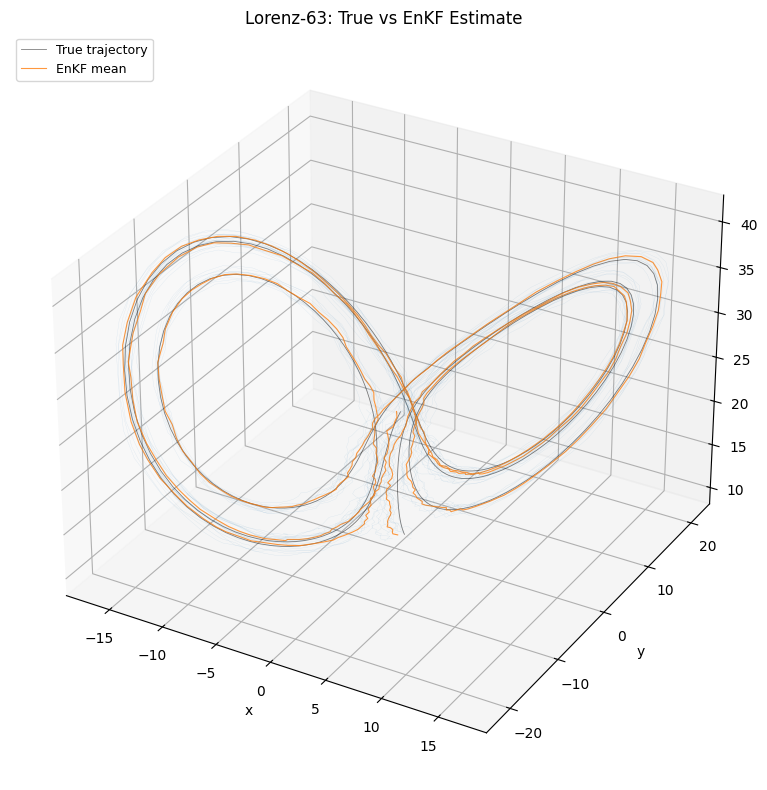

Plot: time series with ensemble spread¶

Each state component over time, showing the true value, ensemble mean, and $\pm 2\sigma$ spread computed from the ensemble.

# Compute ensemble standard deviation at each time step
enkf_std = jnp.std(enkf_ensembles, axis=1)  # (T, 3)

labels = ["x", "y", "z"]
fig, axes = plt.subplots(3, 1, figsize=(12, 8), sharex=True)

for i, (ax, label) in enumerate(zip(axes, labels, strict=True)):
    ax.plot(times, true_states[:, i], "k--", lw=1.5, label="True", zorder=4)
    ax.plot(times, enkf_means[:, i], "C1-", lw=2, label="EnKF mean", zorder=3)
    ax.fill_between(
        times,
        enkf_means[:, i] - 2 * enkf_std[:, i],
        enkf_means[:, i] + 2 * enkf_std[:, i],
        color="C1",
        alpha=0.2,
        label=r"$\pm 2\sigma$",
    )
    if i < 2:
        ax.scatter(
            times,
            observations[:, i],
            s=30,
            c="C0",
            edgecolors="k",
            linewidths=0.5,
            alpha=0.2,
            label="Observations",
            zorder=5,
        )
    ax.set_ylabel(label)
    ax.legend(loc="upper right", fontsize=9, ncol=2)
    ax.grid(True, which="major", alpha=0.3)
    ax.grid(True, which="minor", alpha=0.1)
    ax.minorticks_on()

axes[-1].set_xlabel("Time")
axes[0].set_title("EnKF State Estimates with Ensemble Spread")
plt.tight_layout()
plt.show()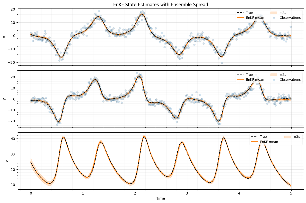

Plot: RMSE over time¶

rmse = jnp.sqrt(jnp.mean((enkf_means - true_states) ** 2, axis=1))

fig, ax = plt.subplots(figsize=(12, 3))
ax.plot(times, rmse, "C3-", lw=2)
ax.set_xlabel("Time")
ax.set_ylabel("RMSE")
ax.set_title("EnKF Root Mean Square Error over Time")
ax.grid(True, which="major", alpha=0.3)
ax.grid(True, which="minor", alpha=0.1)
ax.minorticks_on()
plt.tight_layout()
plt.show()

print(f"Mean RMSE: {jnp.mean(rmse):.3f}")
print(f"Final RMSE: {rmse[-1]:.3f}")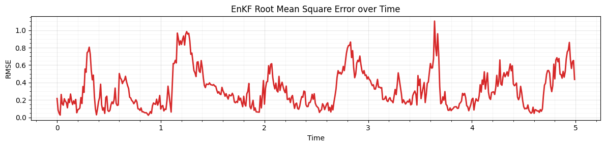

Mean RMSE: 0.320
Final RMSE: 0.435

Summary¶

gaussx.ensemble_covariance(particles) returns a LowRankUpdate operator representing the empirical covariance. This structured representation avoids materializing a full $d \times d$ matrix and enables efficient Woodbury-based solves when the ensemble size $J \ll d$ .
gaussx.ensemble_cross_covariance(particles_theta, particles_G) computes the cross-covariance matrix between two ensembles, giving the $(d_1, d_2)$ array needed for the Kalman gain.
gaussx.joseph_update(P_pred, K, H, R) provides the numerically stable Joseph-form covariance update, guaranteeing symmetry even when the Kalman gain is approximate.
gaussx.process_noise_covariance(A, Pinf) derives the process noise $Q = P_\infty - A P_\infty A^\top$ from a stationary covariance, useful when calibrating a filter from long-run statistics.

Together these primitives let you build ensemble Kalman methods that are fully compatible with JAX transforms (jit, vmap, grad) while preserving structured linear algebra where it matters.

References¶

Evensen, G. (1994). Sequential data assimilation with a nonlinear quasi-geostrophic model using Monte Carlo methods to forecast error statistics. J. Geophys. Res., 99(C5), 10143--10162.
Lorenz, E. N. (1963). Deterministic nonperiodic flow. J. Atmos. Sci., 20(2), 130--141.
Bucy, R. S. & Joseph, P. D. (1968). Filtering for Stochastic Processes with Applications to Guidance. Interscience.
Sarkka, S. (2013). Bayesian Filtering and Smoothing. Cambridge University Press.