Pathwise GP Posterior Sampling

This notebook demonstrates pyrox.gp.PathwiseSampler and pyrox.gp.DecoupledPathwiseSampler — callable posterior function draws via Matheron’s rule. Each sampled path is a single deterministic function that can be evaluated at arbitrary inputs without refactorizing a test-set covariance, which is the enabler for Thompson sampling, Bayesian optimization, and posterior visualization.

What you’ll learn:

The Matheron-rule identity behind PathwiseSampler and why the RFF prior draw matters.
Drawing and evaluating posterior function samples from an exact ConditionedGP.
The sparse / decoupled variant over an SVGP-style inducing set.
A minimal Thompson-sampling loop on a 1D toy objective.

Background¶

Matheron’s rule¶

For a GP prior $f \sim \mathrm{GP}(\mu, k)$ with Gaussian observations $y = f(X) + \varepsilon$ , $\varepsilon \sim \mathcal{N}(0, \sigma^2 I)$ , the posterior sample path admits the Matheron decomposition

\hat{f}_{\mathrm{post}}(\cdot) = \underbrace{\tilde f(\cdot)}_{\text{prior draw}} + \underbrace{k(\cdot, X)\,(K_{XX} + \sigma^2 I)^{-1}\,(y - \tilde f(X) - \tilde\varepsilon)}_{\text{correction}},

((1))

where $\tilde f$ is drawn from the prior and $\tilde\varepsilon \sim \mathcal{N}(0, \sigma^2 I)$ is an independent noise draw at the training inputs. The key insight: if the prior draw $\tilde f$ is represented by a closed-form basis (e.g. random Fourier features), then $\hat f_{\mathrm{post}}$ is a single callable function — evaluate it at any $x_*$ in $\mathcal{O}(F + N)$ without touching $K_{**}$ .

Random Fourier features for the prior draw¶

For a stationary kernel $k(x, x') = \sigma^2 \rho(\|x-x'\|/\ell)$ , Bochner’s theorem gives a spectral density $S(\omega)$ such that

k(x, x') = \sigma^2 \int S(\omega)\,\cos(\omega^\top(x - x'))\,d\omega.

((2))

Sampling $F$ frequencies $\omega_j \sim S$ and phases $b_j \sim \mathrm{Unif}(0, 2\pi)$ ,

\tilde f(x) = \sum_{j=1}^F w_j\,\sqrt{2\sigma^2/F}\,\cos(\omega_j^\top x / \ell + b_j), \qquad w_j \sim \mathcal{N}(0, 1),

((3))

defines a function whose covariance converges to $k$ as $F \to \infty$ . pyrox._basis.draw_rff_cosine_basis is the pure shared primitive that implements this for RBF and Matern kernels; the pathwise samplers call into it.

Sparse / decoupled form¶

For a sparse SparseGPPrior + variational guide $q(u) = \mathcal{N}(m, S)$ over inducing values $u = f(Z)$ , the decoupled Matheron sample is

\hat f_{\mathrm{post}}(x_*) = \tilde f(x_*) + k(x_*, Z)\,K_{ZZ}^{-1}\,(u^{(s)} - \tilde f(Z)),\qquad u^{(s)} \sim q(u).

((4))

DecoupledPathwiseSampler handles WhitenedGuide automatically by unwhitening $v \sim q(v)$ into $u = L_{ZZ} v$ before forming the correction.

Setup¶

import subprocess
import sys


try:
    import google.colab  # noqa: F401

    IN_COLAB = True
except ImportError:
    IN_COLAB = False

if IN_COLAB:
    subprocess.run(
        [
            sys.executable,
            "-m",
            "pip",
            "install",
            "-q",
            "pyrox[colab] @ git+https://github.com/jejjohnson/pyrox@main",
        ],
        check=True,
    )

import warnings


warnings.filterwarnings("ignore", message=r".*IProgress.*")

import jax
import jax.numpy as jnp
import jax.random as jr
import matplotlib.pyplot as plt
import numpyro

from pyrox.gp import (
    RBF,
    DecoupledPathwiseSampler,
    FullRankGuide,
    GPPrior,
    PathwiseSampler,
    SparseGPPrior,
)


jax.config.update("jax_enable_x64", True)

Toy dataset¶

key = jr.PRNGKey(0)

f_true = lambda x: jnp.sin(2.0 * x) + 0.3 * jnp.cos(5.0 * x)

X_train = jnp.concatenate(
    [jnp.linspace(-3.0, -0.5, 10), jnp.linspace(1.5, 3.0, 10)]
).reshape(-1, 1)
noise_std = 0.15
y_train = f_true(X_train.squeeze(-1)) + noise_std * jr.normal(key, (X_train.shape[0],))
X_test = jnp.linspace(-3.5, 3.5, 200).reshape(-1, 1)
noise_var = jnp.array(noise_std**2)

Exact pathwise samples¶

Fit a plain ConditionedGP, then draw 32 callable posterior paths and evaluate them on the dense test grid.

posterior = GPPrior(
    kernel=RBF(init_variance=1.0, init_lengthscale=0.6),
    X=X_train,
    jitter=1e-6,
).condition(y_train, noise_var)

sampler = PathwiseSampler(posterior, n_features=1024)
with numpyro.handlers.seed(rng_seed=0):
    paths = sampler.sample_paths(jr.PRNGKey(1), n_paths=32)
    draws = paths(X_test)  # (32, N_star) — same callable evaluated on the full grid
    mean_star, var_star = posterior.predict(X_test)
std_star = jnp.sqrt(jnp.clip(var_star, min=0.0))

fig, ax = plt.subplots(figsize=(12, 5))
ax.plot(
    X_test.squeeze(),
    f_true(X_test.squeeze()),
    "k--",
    lw=1.5,
    label="True function",
    zorder=5,
)
for draw in draws:
    ax.plot(X_test.squeeze(), draw, color="C0", alpha=0.15, lw=1.0)
ax.plot(
    X_test.squeeze(), mean_star, "C3-", lw=2, label="Analytic posterior mean", zorder=4
)
ax.fill_between(
    X_test.squeeze(),
    mean_star - 2 * std_star,
    mean_star + 2 * std_star,
    color="C3",
    alpha=0.15,
    label=r"$\pm 2\sigma$ (analytic)",
)
ax.scatter(
    X_train.squeeze(),
    y_train,
    s=30,
    c="C1",
    edgecolors="k",
    linewidths=0.5,
    label="Training data",
    zorder=6,
)
ax.set_xlabel("x")
ax.set_ylabel("y")
ax.set_title(
    "Exact GP: 32 pathwise posterior samples (blue) vs. analytic moments (red)"
)
ax.legend(loc="lower left", fontsize=9)
plt.show()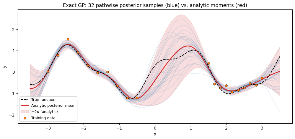

The blue paths are independent callable function draws. Reevaluating the same path on a different input batch gives numerically identical values — a property the analytic predictive moments alone cannot provide without refactorizing a joint test-set covariance.

Sanity check: empirical moments from 512 draws match the analytic posterior.

with numpyro.handlers.seed(rng_seed=0):
    big = PathwiseSampler(posterior, n_features=2048)(
        jr.PRNGKey(2), X_test, n_paths=512
    )
empirical_mean = jnp.mean(big, axis=0)
empirical_std = jnp.std(big, axis=0)

fig, axes = plt.subplots(1, 2, figsize=(14, 4), sharex=True)
axes[0].plot(X_test.squeeze(), empirical_mean, "C0-", lw=2, label="Empirical")
axes[0].plot(X_test.squeeze(), mean_star, "k--", lw=1.5, label="Analytic")
axes[0].set_title("Mean")
axes[0].set_xlabel("x")
axes[0].legend()

axes[1].plot(X_test.squeeze(), empirical_std, "C0-", lw=2, label="Empirical")
axes[1].plot(X_test.squeeze(), std_star, "k--", lw=1.5, label="Analytic")
axes[1].set_title("Standard deviation")
axes[1].set_xlabel("x")
axes[1].legend()
plt.tight_layout()
plt.show()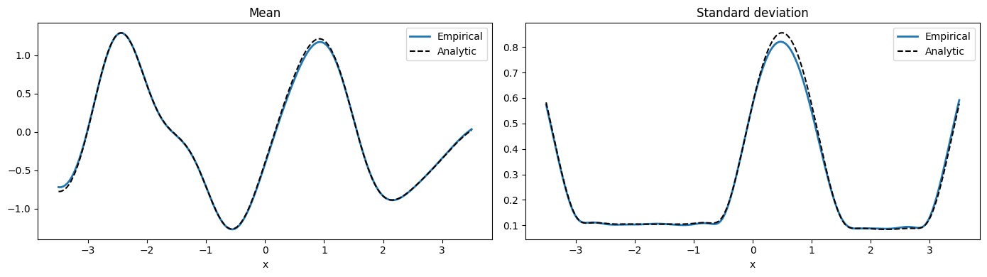

Sparse / decoupled pathwise samples¶

Same story with a sparse GP: a point-inducing SparseGPPrior, a variational guide $q(u) = \mathcal{N}(m, L L^\top)$ , and the decoupled Matheron update. The prior draw reuses the RFF basis; the correction is computed in the inducing-point basis, so the resulting function is callable at arbitrary inputs after a one-time inducing solve.

To give the sampler a realistic guide — instead of a hand-picked mean/covariance with no relation to the data — we set $q(u)$ to the exact conditional $p(u \mid y)$ of the inducing values given the training data. This is the closed-form Bayes-optimal Gaussian over $u$ , and it’s what a fully-converged SVGP guide would match. The resulting decoupled paths should reproduce the exact GP posterior samples up to the RFF + inducing-set approximation.

Z = jnp.linspace(-3.5, 3.5, 20).reshape(-1, 1)
kernel_sparse = RBF(init_variance=1.0, init_lengthscale=0.6)
sparse_prior = SparseGPPrior(kernel=kernel_sparse, Z=Z, jitter=1e-6)

# Closed-form posterior over inducing values u = f(Z) given training data:
# q(u) = p(u | y) = N(K_zx (K_xx + σ² I)⁻¹ y, K_zz − K_zx (K_xx + σ² I)⁻¹ K_xz).
K_xx = kernel_sparse(X_train, X_train) + noise_var * jnp.eye(X_train.shape[0])
K_xx_inv = jnp.linalg.inv(K_xx)
K_zx = kernel_sparse(Z, X_train)
K_zz = kernel_sparse(Z, Z) + 1e-6 * jnp.eye(Z.shape[0])
m_u = K_zx @ K_xx_inv @ y_train
S_u = K_zz - K_zx @ K_xx_inv @ K_zx.T
S_u = 0.5 * (S_u + S_u.T) + 1e-6 * jnp.eye(Z.shape[0])
L_u = jnp.linalg.cholesky(S_u)
guide = FullRankGuide(mean=m_u, scale_tril=L_u)

with numpyro.handlers.seed(rng_seed=0):
    sparse_paths = DecoupledPathwiseSampler(
        sparse_prior, guide, n_features=1024
    ).sample_paths(jr.PRNGKey(3), n_paths=32)
    sparse_draws = sparse_paths(X_test)

fig, ax = plt.subplots(figsize=(12, 5))
for draw in sparse_draws:
    ax.plot(X_test.squeeze(), draw, color="C2", alpha=0.15, lw=1.0)
ax.plot(
    X_test.squeeze(),
    f_true(X_test.squeeze()),
    "k--",
    lw=1.5,
    label="True function",
    zorder=5,
)
ax.plot(
    X_test.squeeze(),
    mean_star,
    "C3-",
    lw=2,
    label="Exact-GP posterior mean (reference)",
    zorder=4,
)
ax.scatter(
    X_train.squeeze(),
    y_train,
    s=30,
    c="C1",
    edgecolors="k",
    linewidths=0.5,
    label="Training data",
    zorder=6,
)
ax.scatter(
    Z.squeeze(),
    m_u,
    s=40,
    c="C2",
    marker="^",
    edgecolors="k",
    linewidths=0.5,
    label=r"Inducing posterior mean $m_u$",
    zorder=6,
)
ax.set_xlabel("x")
ax.set_ylabel("y")
ax.set_title("DecoupledPathwiseSampler: 32 SVGP posterior samples")
ax.legend(loc="lower left", fontsize=9)
plt.show()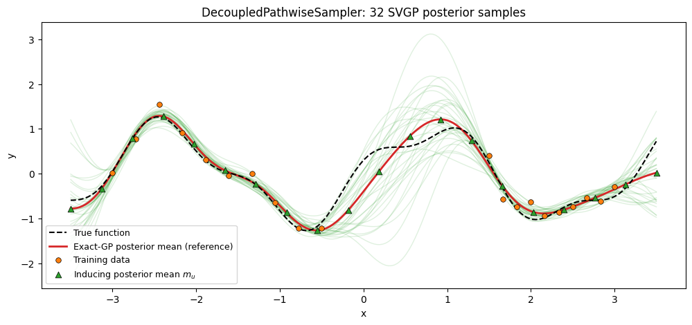

Thompson sampling on a 1D toy¶

The canonical pathwise-sampling use case. At each round:

Draw a single posterior path from the current ConditionedGP.
Pick the argmin of that path (Thompson’s “sample and act” rule for minimization).
Observe the true objective plus noise and condition the GP on the augmented dataset.

Because a sampled path is a single callable function, step 2 is a trivial grid / argmin evaluation — no repeated full-covariance predictives.

def objective(x):
    return (x - 1.7) ** 2 * jnp.cos(3.0 * x) + 0.1 * x


domain = jnp.linspace(-3.0, 3.0, 400).reshape(-1, 1)

# Seed observations.
ts_key = jr.PRNGKey(123)
X_obs = jnp.array([[-2.0], [0.0], [2.5]])
y_obs = objective(X_obs.squeeze(-1)) + 0.05 * jr.normal(ts_key, (X_obs.shape[0],))


def ts_step(X_obs, y_obs, round_key):
    ts_posterior = GPPrior(
        kernel=RBF(init_variance=1.5, init_lengthscale=0.6),
        X=X_obs,
        jitter=1e-6,
    ).condition(y_obs, jnp.array(0.05**2))
    path = PathwiseSampler(ts_posterior, n_features=1024).sample_paths(
        round_key, n_paths=1
    )
    draw = path(domain)[0]  # (N_domain,)
    x_next = domain[jnp.argmin(draw)]  # (1,) — one row of domain
    y_next = objective(x_next) + 0.05 * jr.normal(round_key, (1,))
    return (
        jnp.concatenate([X_obs, x_next[None, :]], axis=0),
        jnp.concatenate([y_obs, y_next], axis=0),
        draw,
    )


rounds = 8
recorded = [(X_obs.copy(), y_obs.copy(), None)]
for r in range(rounds):
    X_obs, y_obs, draw = ts_step(X_obs, y_obs, jr.fold_in(jr.PRNGKey(999), r))
    recorded.append((X_obs.copy(), y_obs.copy(), draw))

fig, axes = plt.subplots(2, 4, figsize=(18, 8), sharex=True, sharey=True)
for ax, (X_step, y_step, draw) in zip(axes.flat, recorded[1:]):
    ax.plot(
        domain.squeeze(),
        objective(domain.squeeze()),
        "k--",
        lw=1.2,
        label="True objective",
    )
    if draw is not None:
        ax.plot(domain.squeeze(), draw, color="C0", lw=1.2, label="Sampled path")
    ax.scatter(
        X_step.squeeze(),
        y_step,
        s=40,
        c="C1",
        edgecolors="k",
        linewidths=0.5,
        label="Observed",
    )
    ax.scatter(
        X_step[-1:].squeeze(),
        y_step[-1:],
        s=120,
        facecolors="none",
        edgecolors="C3",
        linewidths=2.0,
        label="Just picked",
    )
    ax.set_xlabel("x")
for ax in axes[:, 0]:
    ax.set_ylabel("y")
axes[0, 0].legend(loc="upper left", fontsize=8)
plt.suptitle("Thompson sampling: 8 rounds")
plt.tight_layout()
plt.show()

domain_obj = objective(domain.squeeze(-1))
print(f"Best observed value: {float(jnp.min(y_obs)):.3f}")
print(
    f"Argmin (true):       x* = {float(domain.squeeze(-1)[jnp.argmin(domain_obj)]):.3f}"
)
print(f"Argmin (observed):   x  = {float(X_obs.squeeze(-1)[jnp.argmin(y_obs)]):.3f}")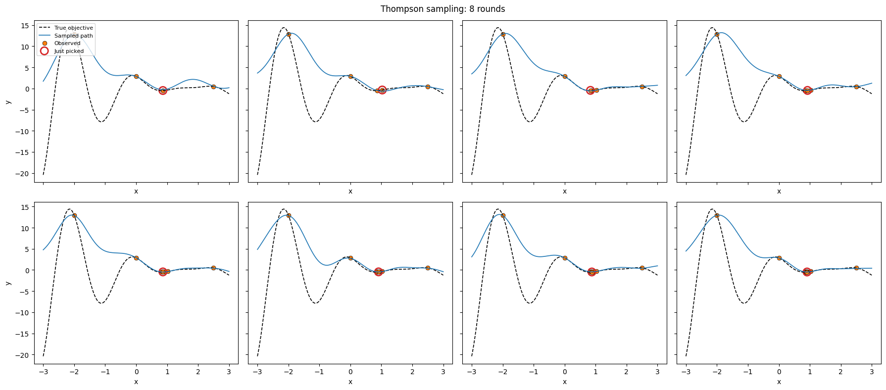

Best observed value: -0.484

Argmin (true):       x* = -3.000
Argmin (observed):   x  = 0.910

Takeaways¶

A pathwise sample is a callable function, not a vector of values — reusable across arbitrary test sets.
PathwiseSampler uses the cached noisy operator from ConditionedGP, so the training Cholesky is shared with the standard predictive path.
DecoupledPathwiseSampler composes with any of the FullRankGuide, MeanFieldGuide, WhitenedGuide, NaturalGuide, DeltaGuide guides; whitened guides are unwhitened automatically.
The shared RFF prior draw lives in pyrox._basis.draw_rff_cosine_basis + evaluate_rff_cosine_paths — the same primitive other posterior-function workflows (custom BO acquisitions, ensembled spectral estimators) can build on directly.