Ensemble primitives

Background — Bayesian regression and ensemble MAP¶

Bayes’ rule for parameters¶

Given an i.i.d. dataset $\mathcal{D} = \{(x_i, y_i)\}_{i=1}^N$, a likelihood model $p(y \mid x, \theta)$ and a prior $p(\theta)$, Bayes’ rule for the model parameters reads

Two facts about the right-hand side determine everything below: (1) the numerator is cheap (one likelihood evaluation per data point and one prior evaluation), and (2) the denominator $p(\mathcal{D})$ — the marginal likelihood — is intractable except for conjugate models. Every approximate-inference method we use is, at heart, a way to avoid computing $p(\mathcal{D})$.

Log-posterior decomposition¶

Taking logs and dropping the $\log p(\mathcal{D})$ constant (which doesn’t depend on θ and so doesn’t move under any optimizer or sampler), the log-posterior splits into a likelihood term and a prior term:

Three classical estimators flow from different ways of using this functional:

• MLE — maximize $\ell(\theta)$ alone. Drops the prior; equivalent to uniform $p(\theta)$.
• MAP — maximize $\ell(\theta) + \log p(\theta)$. The mode of the posterior; the prior acts as a regularizer.
• Full Bayes — characterize the whole posterior $p(\theta \mid \mathcal{D})$, typically by samples (HMC) or a variational surrogate (VI).

The pyrox.inference primitives expose prior_weight so you can interpolate between MLE (prior_weight=0) and MAP (prior_weight=1); fractional values give a tempered MAP with a softer prior.

The Gaussian likelihood + Gaussian prior special case¶

When $p(y \mid x, \theta) = \mathcal{N}(y \mid f_\theta(x), \sigma^2)$ and $p(\theta) = \mathcal{N}(\theta \mid 0, \tau^2 I)$, the log-joint reads

Maximizing it (MAP) is exactly ridge regression with regularization strength $\lambda = \sigma^2 / \tau^2$. So Pattern A below — Gaussian likelihood, standard-normal prior on every weight, Adam — is L2-regularized least-squares with a deep network as the regression function and SGD as the solver.

Predictive distribution and Monte-Carlo evaluation¶

Once we have either the posterior $p(\theta \mid \mathcal{D})$ or an approximation $q(\theta)$, predictions for a fresh input $x^*$ come from the posterior predictive:

The integral is intractable in general but the Monte-Carlo estimator on the right is unbiased for any sampler that produces $\theta^{(s)}$ from the posterior.

Ensemble MAP as a Dirac mixture posterior¶

An ensemble of $E$ MAP estimates is $E$ independent SGD descents of $-\log p(\theta, \mathcal{D})$ from $E$ different random initializations $\theta_e^{(0)} \sim p_{\text{init}}(\cdot)$. Each descent converges (typically) to a different local mode $\hat\theta_e$. Treating the ensemble as a uniform mixture of point masses,

the posterior-predictive Monte-Carlo estimator collapses to

This is the deep-ensembles estimator (Lakshminarayanan et al., 2017) — the cheapest useful uncertainty estimator one can build for a neural model. The between-member variance $\mathrm{Var}_e[\,\mathbb{E}_{p(y^*|\,x^*,\hat\theta_e)}[y^*]\,]$ is taken as a proxy for epistemic uncertainty (uncertainty about which mode is right).

Mini-batch SGD as an unbiased estimator¶

When $N$ is large, evaluating $\sum_{i=1}^N \log p(y_i \mid x_i, \theta)$ on every step is expensive. We replace it with a uniformly-sampled mini-batch $B \subset \{1,\dots,N\}$ of size $|B|$ and rescale:

The $N/|B|$ factor (the scale argument to ensemble_step) ensures $\mathbb{E}_B[\widehat{\mathcal{L}}(\theta)] = -\log p(\theta, \mathcal{D})$, so the SGD step direction is unbiased for the full-data MAP gradient.

What ensemble_step does¶

Putting it together, pyrox.inference.ensemble_step(state, x_batch, y_batch, *, log_joint, optimizer, prior_weight, scale) does exactly one optimizer step on $\widehat{\mathcal{L}}$ for every member, in parallel via eqx.filter_vmap. Concretely, per member $e$:

1. Compute $(\ell_e, \pi_e) = \texttt{log\_joint}(\theta_e, x_B, y_B)$ where $\ell_e$ is the batched log-likelihood and $\pi_e$ is the log-prior.
2. Form $\mathcal{L}_e = -\,\texttt{scale}\cdot \ell_e - \texttt{prior\_weight}\cdot \pi_e$.
3. Compute $\nabla_{\theta_e} \mathcal{L}_e$ via eqx.filter_value_and_grad (only differentiates wrt the inexact-array leaves of $\theta_e$).
4. Apply one optax step: $\theta_e \leftarrow \theta_e + \texttt{optimizer.update}(\nabla \mathcal{L}_e)$.

Inputs:

• state — EnsembleState(params, opt_state) whose array leaves carry a leading $(E,)$ axis.
• log_joint(params, x_batch, y_batch) -> (loglik, logprior) — your scalar log-densities.
• optimizer — any optax.GradientTransformation.
• scale = N / |B| — unbiases the mini-batch gradient.
• prior_weight — 0 recovers MLE; 1 recovers MAP; fractional values give a tempered MAP.

Returns (new_state, per_member_losses: shape (E,)). That’s the entire contract — everything else (batching, schedules, callbacks, early stopping) is yours.

Setup¶

Problem setup — the sinc dataset¶

A 1D regression target $y = \mathrm{sinc}(x/\pi) + \epsilon$ on $[-10, 10]$ with $\epsilon \sim \mathcal{N}(0, 0.1)$. Eighty noisy training points, two hundred dense test points for evaluation. We also generate a noisy test sample by adding fresh observation noise to the dense grid — that is what we will score the predictive distribution against, since $y_{\text{truth}}$ has zero observation noise and so cannot validate the aleatoric component of the predictive.

Goodness-of-fit metrics for a Bayesian regressor¶

A single R² over the noiseless truth is a thin reading of model quality — it ignores predictive uncertainty entirely. For a probabilistic regressor we want to assess (1) the mean prediction’s accuracy, (2) whether the predictive intervals cover the truth at the nominal rate (calibration), and (3) whether those intervals are as tight as possible given they are calibrated (sharpness). The metrics below combine to do that.

Notation. Let $\{f_m\}_{m=1}^M$ be the per-member mean predictions on the test grid (so $M = E$ for a MAP ensemble, or $M = E \cdot S$ for a VI ensemble that drew $S$ posterior samples per member). The posterior-predictive at $x^*_i$ is the equally-weighted Gaussian mixture

whose variance decomposes as

RMSE — the root-mean-squared error of the mean prediction $\bar f$ against (a) the noiseless truth $y_{\text{truth}}$ and (b) the noisy observation $y_{\text{obs}}$. Even an oracle predictor cannot beat σ on the noisy version, so RMSE-obs $\approx \sigma$ is best-possible.

NLL (negative log predictive density) — proper scoring rule:

Lower is better. NLL penalizes both miscalibration and inaccuracy with one number; it is the gold-standard metric for probabilistic regression.

Coverage at level α — fraction of test observations $y^{\text{obs}}_i$ that fall inside the central α-credible interval of the predictive distribution. A perfectly calibrated model has empirical coverage = α at every α. Under-coverage (empirical $<$ nominal) is overconfidence; over-coverage is underconfidence.

Sharpness at level α — mean width of the central α-credible interval. Conditional on calibration, lower sharpness is better (tighter intervals = more informative). For an uncalibrated model, however, sharpness alone is misleading — a model that always predicts $[-\infty, +\infty]$ has perfect coverage at any level but is useless.

Calibration curve — empirical coverage vs nominal α over $\alpha \in (0, 1)$. The ideal trace is the diagonal; consistent under-the-diagonal means systematic overconfidence.

We compute everything by Monte-Carlo sampling from the predictive mixture so the same code path handles MAP point-mass mixtures and VI continuous-distribution mixtures uniformly.

A shared MLP architecture¶

All three patterns fit the same architecture: a 1→32→32→1 MLP with tanh activations. Patterns A and B carry the model as an eqx.nn.MLP module; pattern C re-expresses the same architecture as a NumPyro model so it composes with log_density.

Pattern A — From scratch (raw log-joint, manual loop)¶

The most direct way to use the primitives. We supply:

1. An init_fn(key) -> params that returns one eqx.nn.MLP per ensemble member.
2. A log_joint(params, x_batch, y_batch) -> (loglik, logprior) with a Gaussian likelihood (variance SIGMA²) and a standard-normal prior on every weight leaf.
3. An optax.adam(5e-3) optimizer.

Then we call ensemble_init once, jit-wrap ensemble_step, and run a Python loop. The Python loop is what makes the cost of jit’ing one step (instead of lax.scan-ing the whole training) negligible — eqx.filter_jit traces once, every subsequent call dispatches the cached XLA executable.

Math: Gaussian likelihood + standard-normal weight prior¶

Let $f_\theta : \mathbb{R} \to \mathbb{R}$ be the MLP and $\theta = (W_\ell, b_\ell)_{\ell=1}^L$ collect all of its weights and biases. Modeling each observation as $y_i \mid x_i, \theta \sim \mathcal{N}\bigl(f_\theta(x_i),\, \sigma^2\bigr)$ with known σ, the log-likelihood for a batch $B$ is

The constant in θ doesn’t move under any optimizer, so we drop it in the implementation. Putting an isotropic standard-normal prior on every weight, $\theta \sim \mathcal{N}(0, I)$, the log-prior is

which is exactly the L2-regularization functional. The MAP gradient combines the two:

Adam (Kingma & Ba, 2015) advances θ along an exponentially-weighted estimate of this gradient with per-coordinate learning rates derived from the second moment. Crucially we don’t write any of this update by hand — optax.adam(5e-3) is the entire implementation, and eqx.filter_value_and_grad only differentiates wrt the inexact-array leaves of the MLP (skipping the jax.nn.tanh activation function reference, etc.).

Pattern B — Optax composition + early stopping¶

The primitives accept any optax.GradientTransformation, so we can compose schedules and clipping freely. Here we stack clip_by_global_norm + adamw + warmup_cosine_decay. We also use the manual Python loop’s flexibility to early-stop when the average loss plateaus for patience epochs — something the one-shot EnsembleMAP.run (which lives inside lax.scan) can’t express.

Math: schedule, clipping, AdamW, and early stopping as regularizers¶

Warmup-cosine schedule. Adam’s per-coordinate learning rate is multiplied by a global $\eta_t$ that ramps linearly from $\eta_0$ to $\eta_{\max}$ over the first $T_w$ steps and then decays as a half-cosine to $\eta_\infty$:

The warmup avoids the catastrophic first-step blowup that hits randomly-initialized networks at high LR; the cosine tail is empirically the most robust late-training schedule for SGD-with-momentum-style methods.

Global-norm clipping. Before each Adam step, the raw gradient $g$ is rescaled if its global norm exceeds a threshold $c$:

This bounds the maximum step size in raw-gradient units, which prevents single bad batches (e.g. an outlier) from kicking the parameters out of a basin. We use $c = 1$.

AdamW vs Adam. AdamW (Loshchilov & Hutter, 2019) decouples the L2 weight-decay term from the Adam moment estimates: instead of folding θ into the gradient (which makes the decay rate effective scale with the second-moment estimate), it applies $\theta \leftarrow (1 - \eta_t \lambda)\,\theta$ as a separate post-step update. We pass weight_decay=0.0 here because the L2 penalty already lives in our log_joint via the standard-normal prior — AdamW’s slot is on standby for problems where you’d rather control regularization through the optimizer than through the prior.

Early stopping as implicit regularization. Stopping at step $t^* < T$ caps the path length the optimizer can travel from $\theta_0$. For convex losses, this gives an effective regularization equivalent to a Tikhonov penalty proportional to $1/\eta t^*$ (Yao, Rosasco, Caponnetto, 2007). For non-convex losses there is no clean closed form, but the empirical effect is the same: less time on $\widehat{\mathcal{L}}$ means less overfitting to the training noise, at some cost in train R². The trade-off shows up in the comparison table below — Pattern B’s early-stop fit lands at slightly lower train R² than Pattern A’s full 1500-epoch fit, but with sometimes-better generalization.

Pattern C — NumPyro log_density (wrap an existing NumPyro model)¶

If you already have a NumPyro model — for instance because you want to reuse the same model with NUTS later — you don’t need to rewrite it as a log_joint. NumPyro ships numpyro.infer.util.log_density(model, args, kwargs, params) which evaluates the full log joint (likelihood + prior) for a flat dictionary of latent values. We wrap that in a tiny adapter that returns (full_joint, 0) and tell ensemble_step to skip the prior term (prior_weight=0) so we don’t double-count.

The model below is the same MLP-with-Gaussian-priors architecture, just expressed as a chain of numpyro.sample sites with names W1, b1, ..., b3. The init function returns a dict matching those names, drawn from priors at init time.

Math: what log_density computes and why prior_weight=0¶

Given a NumPyro model — a Python function that calls numpyro.sample to declare latent and observed sites — numpyro.infer.util.log_density(model, args, kwargs, params) runs the model under a substitute handler that replaces every latent site $\theta_k$ with the corresponding entry of params, traces the model to collect every site (latent and observed), and returns

Notice this is the complete log joint — it already contains both the prior and the likelihood. If we passed it through to ensemble_step as the likelihood term and let prior_weight=1 add another log_joint(...)[1] on top, we would either double-count the prior (if the user split it) or do nothing (if the user returned 0 for the prior term). The cleaner contract is: hand log_density’s scalar output to the likelihood slot and set prior_weight=0. With scale=1 and prior_weight=0, ensemble_step minimizes exactly $-\log p(\theta, y \mid x)$, which is the MAP objective.

Tempered MAP. If you want a tempered MAP — say, downweight the prior by $\beta < 1$ — you’d need to split log_density’s output into prior and likelihood pieces yourself. The cleanest way is to evaluate the model under numpyro.handlers.substitute(numpyro.handlers.trace(...)) and split sites by the is_observed flag; that’s the same pattern used internally by numpyro.infer.SVI and is described in the next tutorial.

Why this is useful. It means the same NumPyro model can drive (1) NUTS via numpyro.infer.MCMC, (2) full-Bayes VI via numpyro.infer.SVI, and (3) ensemble MAP via this Pattern C. Different inference paradigms, one model spec — which is the whole reason NumPyro models are written as functions in the first place.

Goodness-of-fit comparison¶

Now we evaluate all three predictive distributions against the noisy test observations. The figure below shows two panels per pattern: (top) the predictive mean and the full posterior-predictive 95% band (epistemic + aleatoric), with the noisy test observations plotted; (bottom) the calibration curve, comparing empirical coverage against nominal coverage at $\alpha = 0.05, 0.1, \dots, 0.95$. A perfectly calibrated model traces the diagonal; below the diagonal means overconfident, above means underconfident.

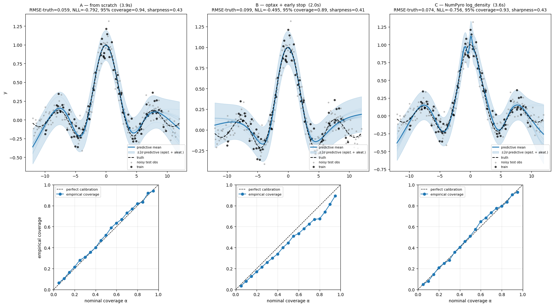
Summary table¶

• RMSE-truth — root mean squared error of the predictive mean against the noiseless truth. Pure accuracy of $\bar f$.
• RMSE-obs — root mean squared error against the noisy observations. Floor is $\sigma = 0.1$ (the irreducible noise).
• NLL — negative log predictive density of the noisy test observations under the mixture-of-Gaussians predictive. Lower is better. The oracle predictor (perfect $f$, known σ) gets NLL $= \tfrac{1}{2}\log(2\pi\sigma^2) + \tfrac{1}{2} \approx -0.88$.
• 95% coverage — fraction of noisy test points inside the central 95% predictive interval. Calibrated $\Rightarrow$ 0.95.
• Sharpness@95 — mean width of the central 95% predictive interval. Lower is better given calibration. With $\sigma = 0.1$, an oracle predictor’s 95% interval has width $\approx 4\sigma = 0.4$.

Takeaways¶

• The primitives are minimal but composable. ensemble_init + ensemble_step is the entire mandatory surface; everything else (the optimizer, the loop, the log-joint origin) is your decision.
• Pattern A is the right starting point when you want to understand exactly what’s happening. No optax magic, no NumPyro, no schedules.
• Pattern B unlocks anything that needs Python control flow: early stopping, adaptive schedules, callbacks for logging or visualization, custom batching strategies. The price is that you can’t lax.scan over a Python if/break, so you trade some speed for control.
• Pattern C is the bridge to existing NumPyro models. Anything you can express as a numpyro model plays nicely with the primitives via log_density. This is also how you’d run NUTS and an ensemble MAP on the same model — write the model once, point both inference paths at it.
• All three are point-mass MAP ensembles. Their predictive variance is $\mathrm{Var}_{\text{epist}} + \sigma^2$, where the epistemic term is typically much smaller than $\sigma^2$ inside the training range — so the bands are dominated by aleatoric noise there. In extrapolation regions ($|x| > 10$) the epistemic term grows, but only modestly, because all members were initialized in similar basins. To get true posterior-predictive uncertainty (especially in extrapolation), see the runner tutorial’s EnsembleVI example.
• When to step up: if you don’t need any of the manual-loop superpowers, the higher-level EnsembleMAP runner is faster (it lax.scans the loop) and shorter to write.