Bayesian Linear Regression with Precision Parameterization
This notebook demonstrates gaussx.MultivariateNormalPrecision in a
NumPyro model for Bayesian linear regression. The precision
parameterization is natural when:
- The prior is specified via a precision matrix (e.g. ridge regularization, Gaussian Markov random fields)
- You want to perform conjugate updates by adding precision matrices directly
- The posterior precision has structure you want to preserve (e.g. banded, sparse, Kronecker)
What you’ll learn:
- Bayesian linear regression with a precision-parameterized prior
- Analytic conjugate posterior in precision form
- Using
MultivariateNormalPrecisionin a NumPyro model with MCMC - Comparing MCMC posterior against the analytic solution
- Posterior predictive with uncertainty quantification
Setup
from __future__ import annotations

import warnings


warnings.filterwarnings("ignore", message=r".*IProgress.*")

import jax
import jax.numpy as jnp
import lineax as lx
import matplotlib.pyplot as plt
import numpyro
import numpyro.distributions as dist
from numpyro.infer import MCMC, NUTS

import gaussx


jax.config.update("jax_enable_x64", True)
Background
In Bayesian linear regression with known noise variance :
With a Gaussian prior specified via precision , the posterior is:
where:
The posterior precision is the sum of prior precision and data precision -- this additivity is why precision parameterization is natural for conjugate updates.
The precision form arises naturally in Gaussian Markov random fields
(GMRFs) where the precision matrix is sparse (typically banded or
block-tridiagonal), encoding conditional independence structure. In
spatial statistics, the SPDE approach (Lindgren et al., 2011) constructs
a GMRF approximation to a Matern GP, where the precision is a sparse
matrix defined by the finite element mesh. gaussx’s
MultivariateNormalPrecision can work with structured precision
operators (banded, block-diagonal, Kronecker) for efficient inference
in these models.
Generate data
We create a polynomial regression problem with known true weights.
key = jax.random.PRNGKey(0)
n = 50
noise_std = 0.5
degree = 5

# True weights
w_true = jnp.array([0.5, -1.2, 0.3, 0.8, -0.4, 0.1])

# Design matrix: polynomial features [1, x, x^2, ..., x^degree]
key, subkey = jax.random.split(key)
x_train = jnp.sort(jax.random.uniform(subkey, (n,), minval=-2, maxval=2))
X_train = jnp.column_stack([x_train**p for p in range(degree + 1)])

# Observations
key, subkey = jax.random.split(key)
y_train = X_train @ w_true + noise_std * jax.random.normal(subkey, (n,))

# Test grid
x_test = jnp.linspace(-2.5, 2.5, 200)
X_test = jnp.column_stack([x_test**p for p in range(degree + 1)])

d = degree + 1
print(f"Design matrix shape: {X_train.shape}")
print(f"True weights: {w_true}")
Design matrix shape: (50, 6)
True weights: [ 0.5 -1.2 0.3 0.8 -0.4 0.1]
Analytic posterior (conjugate)
We compute the exact posterior using the conjugate precision-form update.
# Prior: isotropic precision (ridge regularization)
alpha = 1.0  # prior precision scalar
Lambda_0 = alpha * jnp.eye(d)

# Data precision contribution
Lambda_data = (1 / noise_std**2) * X_train.T @ X_train

# Posterior precision and mean
Lambda_post = Lambda_0 + Lambda_data
mu_post = jnp.linalg.solve(Lambda_post, (1 / noise_std**2) * X_train.T @ y_train)
Sigma_post = jnp.linalg.inv(Lambda_post)

print("Posterior precision (diagonal):", jnp.diag(Lambda_post))
print("Posterior mean:", mu_post)
print("True weights:  ", w_true)
Posterior precision (diagonal): [ 201. 254.39197138 549.16875 1462.54311184
4294.27361813 13305.72205558]
Posterior mean: [ 0.59125703 -1.0474102 0.17119962 0.55799098 -0.36153802 0.16429194]
True weights: [ 0.5 -1.2 0.3 0.8 -0.4 0.1]
NumPyro model with precision prior
We define the model using gaussx.MultivariateNormalPrecision for
the prior on weights. This directly encodes the ridge
regularization as a precision matrix.
def blr_model(X, noise_std, y=None):
    d = X.shape[1]

    # Prior: w ~ N(0, Lambda_0^{-1}) with Lambda_0 = alpha * I
    Lambda_0 = alpha * jnp.eye(d)
    Lambda_0_op = lx.MatrixLinearOperator(Lambda_0, lx.positive_semidefinite_tag)
    w = numpyro.sample(
        "w", gaussx.MultivariateNormalPrecision(jnp.zeros(d), Lambda_0_op)
    )

    # Likelihood: y | w ~ N(Xw, sigma^2 I)
    mu = X @ w
    with numpyro.plate("data", X.shape[0]):
        numpyro.sample("obs", dist.Normal(mu, noise_std), obs=y)
Run NUTS
NumPyro’s NUTS sampler works directly with
MultivariateNormalPrecision — the log-prob and its gradients
are computed via gaussx structural dispatch.
kernel = NUTS(blr_model)
mcmc = MCMC(kernel, num_warmup=500, num_samples=1000, progress_bar=False)
mcmc.run(jax.random.PRNGKey(1), X_train, noise_std, y=y_train)
mcmc.print_summary()
                mean       std    median      5.0%     95.0%     n_eff     r_hat
      w[0]      0.59      0.17      0.59      0.28      0.85    272.51      1.01
      w[1]     -1.04      0.26     -1.04     -1.46     -0.63    217.18      1.03
      w[2]      0.18      0.30      0.17     -0.36      0.63    230.31      1.01
      w[3]      0.55      0.31      0.56      0.04      1.02    195.42      1.03
      w[4]     -0.37      0.09     -0.36     -0.52     -0.23    238.59      1.01
      w[5]      0.16      0.08      0.16      0.04      0.29    204.08      1.03

Number of divergences: 0
w_samples = mcmc.get_samples()["w"]
print("MCMC weight samples shape:", w_samples.shape)
MCMC weight samples shape: (1000, 6)
Compare MCMC vs analytic posterior
The MCMC samples should match the analytic conjugate posterior. We compare marginal distributions for each weight.
fig, axes = plt.subplots(2, 3, figsize=(14, 7))

for i, ax in enumerate(axes.flat):
    # MCMC histogram
    ax.hist(
        w_samples[:, i],
        bins=35,
        density=True,
        alpha=0.6,
        color="steelblue",
        label="MCMC",
    )

    # Analytic posterior
    w_grid = jnp.linspace(
        mu_post[i] - 4 * jnp.sqrt(Sigma_post[i, i]),
        mu_post[i] + 4 * jnp.sqrt(Sigma_post[i, i]),
        200,
    )
    pdf = jnp.exp(dist.Normal(mu_post[i], jnp.sqrt(Sigma_post[i, i])).log_prob(w_grid))
    ax.plot(w_grid, pdf, "C3-", lw=2, label="Analytic")

    # True value
    ax.axvline(w_true[i], color="k", ls="--", lw=1.5, label="True")

    ax.set_title(f"$w_{i}$")
    if i == 0:
        ax.legend(fontsize=9)
    ax.grid(True, which="major", alpha=0.3)
    ax.grid(True, which="minor", alpha=0.1)
    ax.minorticks_on()

fig.suptitle("MCMC vs Analytic Posterior (per weight)", fontsize=13)
plt.tight_layout()
plt.show()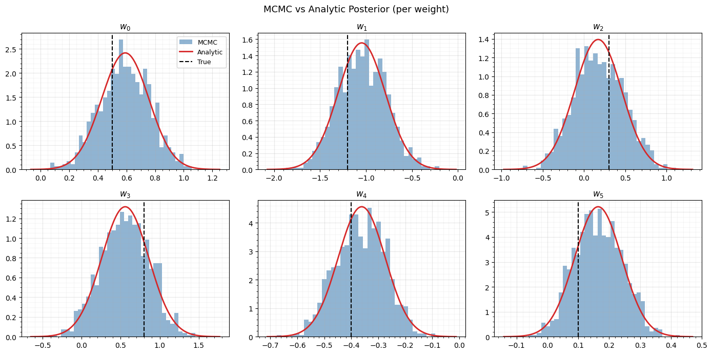
Posterior predictive
We compute the predictive distribution by pushing MCMC weight samples through the model.
# Predictive mean for each sample
y_pred = w_samples @ X_test.T  # (n_samples, n_test)

pred_mean = jnp.mean(y_pred, axis=0)
# Total predictive std: epistemic (weight uncertainty) + aleatoric (noise)
pred_std = jnp.sqrt(jnp.var(y_pred, axis=0) + noise_std**2)

# Also compute analytic predictive
analytic_mean = X_test @ mu_post
analytic_var = jnp.sum(X_test @ Sigma_post * X_test, axis=1) + noise_std**2
analytic_std = jnp.sqrt(analytic_var)

print(f"MCMC pred mean shape: {pred_mean.shape}")
print(f"Analytic pred mean shape: {analytic_mean.shape}")
MCMC pred mean shape: (200,)
Analytic pred mean shape: (200,)
Plot predictions
The MCMC posterior predictive should closely match the analytic solution. Both include observation noise in the uncertainty bands.
fig, ax = plt.subplots(figsize=(12, 5))

# True function
y_true_test = X_test @ w_true
ax.plot(x_test, y_true_test, "k--", lw=1.5, label="True function", zorder=4)

# MCMC predictive
ax.plot(x_test, pred_mean, "C0-", lw=2, label="MCMC mean", zorder=3)
ax.fill_between(
    x_test,
    pred_mean - 2 * pred_std,
    pred_mean + 2 * pred_std,
    color="C0",
    alpha=0.15,
    label=r"MCMC $\pm 2\sigma$",
)

# Analytic predictive
ax.plot(x_test, analytic_mean, "C3--", lw=1.5, label="Analytic mean", zorder=3)
ax.fill_between(
    x_test,
    analytic_mean - 2 * analytic_std,
    analytic_mean + 2 * analytic_std,
    color="C3",
    alpha=0.1,
    label=r"Analytic $\pm 2\sigma$",
)

# Training data
ax.scatter(
    x_train,
    y_train,
    s=30,
    c="C1",
    edgecolors="k",
    linewidths=0.5,
    label="Training data",
    zorder=5,
)

ax.set_xlabel("x")
ax.set_ylabel("y")
ax.set_title("Bayesian Linear Regression: MCMC vs Analytic Posterior")
ax.legend(loc="upper left", fontsize=9, ncol=2)
ax.set_ylim(-5, 5)
ax.grid(True, which="major", alpha=0.3)
ax.grid(True, which="minor", alpha=0.1)
ax.minorticks_on()
plt.tight_layout()
plt.show()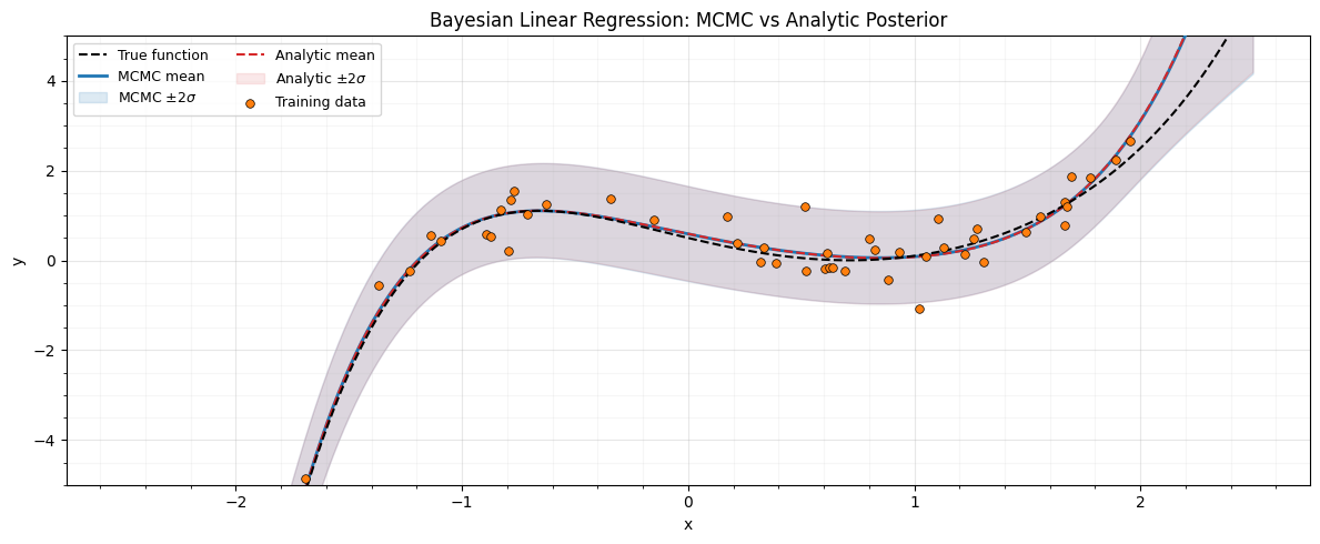
Precision additivity
The key advantage of precision parameterization: posterior precision = prior precision + data precision. Let’s verify this with gaussx.
Each observation adds information (in the Fisher sense) to the posterior. The posterior precision directly reflects this: the total information is the sum of prior information and data information. This additivity is the defining property of the natural parameters of the exponential family.
# Build operators
Lambda_0_op = lx.MatrixLinearOperator(Lambda_0, lx.positive_semidefinite_tag)
Lambda_data_op = lx.MatrixLinearOperator(Lambda_data, lx.positive_semidefinite_tag)
Lambda_post_op = lx.MatrixLinearOperator(Lambda_post, lx.positive_semidefinite_tag)

# Prior
d_prior = gaussx.MultivariateNormalPrecision(jnp.zeros(d), Lambda_0_op)
print("Prior entropy:", d_prior.entropy())

# Posterior
d_post = gaussx.MultivariateNormalPrecision(mu_post, Lambda_post_op)
print("Posterior entropy:", d_post.entropy())

# Entropy should decrease (more information)
print("Entropy decreased:", float(d_prior.entropy()) > float(d_post.entropy()))

# Verify log-prob at posterior mean
print("log p(mu_post | posterior):", d_post.log_prob(mu_post))
Prior entropy: 8.513631199228037
Posterior entropy: -7.486669349647968
Entropy decreased: True
log p(mu_post | posterior): 10.486669349647968
Summary
gaussx.MultivariateNormalPrecisionnaturally encodes ridge regularization and conjugate Bayesian updates.- It plugs directly into NumPyro models — NUTS computes gradients through the precision-parameterized log-prob.
- For linear-Gaussian models, the MCMC posterior matches the analytic conjugate solution, validating the implementation.
- Precision additivity () makes sequential updates trivial — just add precision operators.
- The same pattern extends to structured precisions (banded, Kronecker, block-diagonal) for scalable models like GMRFs.
References
- Bishop, C. M. (2006). Pattern Recognition and Machine Learning. Springer. (Section 3.3 on Bayesian linear regression)
- Lindgren, F., Rue, H., & Lindstrom, J. (2011). An explicit link between Gaussian fields and Gaussian Markov random fields: the stochastic partial differential equation approach. JRSS-B, 73(4), 423--498.
- Rue, H. & Held, L. (2005). Gaussian Markov Random Fields: Theory and Applications. Chapman & Hall/CRC.