GP on a 2D Grid with Kronecker Structure

When data lives on a regular grid, the kernel matrix factorizes as $K = K_x \otimes K_y$ . This enables GP inference on grids with thousands of points that would be intractable with a dense kernel.

This example fits a 2D GP to noisy observations on a grid using Kronecker structure for solve, logdet, and prediction.

Background¶

When inputs lie on a Cartesian product grid $\mathcal{X} = \{x_1, \ldots, x_{n_1}\} \times \{y_1, \ldots, y_{n_2}\}$ and the kernel is separable,

k\bigl((x,y),(x',y')\bigr) = k_x(x,x')\, k_y(y,y'),

((1))

the kernel matrix factorizes as a Kronecker product $K = K_x \otimes K_y$ where $K_x \in \mathbb{R}^{n_1 \times n_1}$ and $K_y \in \mathbb{R}^{n_2 \times n_2}$ . With $N = n_1 n_2$ , this reduces:

Storage from $O(N^2)$ to $O(n_1^2 + n_2^2)$ .
Solve from $O(N^3)$ to $O(n_1^3 + n_2^3)$ .
Log-determinant via $\log|K_x \otimes K_y| = n_2 \log|K_x| + n_1 \log|K_y|$ .

These savings make GP inference feasible on grids with thousands of points that would be intractable with a dense kernel matrix. See Saatci (2012) for a comprehensive treatment and Gilboa et al. (2015) for extensions to higher-dimensional grids.

from __future__ import annotations

import warnings


warnings.filterwarnings("ignore", message=r".*IProgress.*")

import jax
import jax.numpy as jnp
import lineax as lx
import matplotlib.pyplot as plt

import gaussx


jax.config.update("jax_enable_x64", True)

Generate 2D grid data¶

# Grid
nx, ny = 15, 15
N = nx * ny
x = jnp.linspace(0, 4, nx)
y = jnp.linspace(0, 4, ny)
xx, yy = jnp.meshgrid(x, y, indexing="ij")


# True function: a smooth 2D surface
def f_true(x, y):
    return jnp.sin(x) * jnp.cos(1.5 * y)


z_true = f_true(xx, yy)

# Noisy observations
noise_std = 0.15
key = jax.random.PRNGKey(7)
z_obs = z_true + noise_std * jax.random.normal(key, z_true.shape)

print(f"Grid: {nx}x{ny} = {N} points")

Grid: 15x15 = 225 points

fig, axes = plt.subplots(1, 2, figsize=(10, 4))
im0 = axes[0].pcolormesh(xx, yy, z_true, cmap="RdBu_r", shading="auto")
axes[0].set_title("True function")
plt.colorbar(im0, ax=axes[0])

im1 = axes[1].pcolormesh(xx, yy, z_obs, cmap="RdBu_r", shading="auto")
axes[1].set_title(f"Noisy observations ($\\sigma$={noise_std})")
plt.colorbar(im1, ax=axes[1])

for ax in axes:
    ax.set_xlabel("x")
    ax.set_ylabel("y")
    ax.set_aspect("equal")

plt.tight_layout()
plt.show()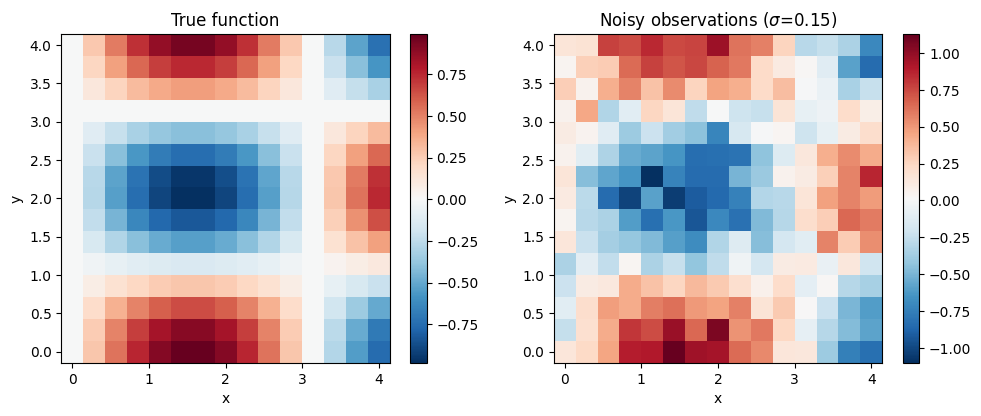

Build Kronecker kernel¶

Separable RBF: $k((x_1,y_1), (x_2,y_2)) = k_x(x_1,x_2) \cdot k_y(y_1,y_2)$

Separability holds for any product of 1D stationary kernels (RBF, Matern, periodic). For non-separable kernels, sums of Kronecker products $\sum_r K_x^{(r)} \otimes K_y^{(r)}$ can be used as approximations.

def rbf_1d(coords, lengthscale, variance):
    sq_dist = (coords[:, None] - coords[None, :]) ** 2
    return variance * jnp.exp(-0.5 * sq_dist / lengthscale**2)


ls_x, ls_y = 1.0, 1.0
var_x, var_y = 1.0, 1.0
noise_var = noise_std**2

Kx = rbf_1d(x, ls_x, var_x)
Ky = rbf_1d(y, ls_y, var_y)

Kx_op = lx.MatrixLinearOperator(Kx, lx.positive_semidefinite_tag)
Ky_op = lx.MatrixLinearOperator(Ky, lx.positive_semidefinite_tag)

# Full kernel: Kx kron Ky + noise * I
K_kron = gaussx.Kronecker(Kx_op, Ky_op)

print(f"Kronecker kernel: {K_kron.in_size()}x{K_kron.out_size()}")
print(f"Storage: {nx}x{nx} + {ny}x{ny} = {nx**2 + ny**2}")
print(f"Dense would be: {N}x{N} = {N**2:,}")

Kronecker kernel: 225x225
Storage: 15x15 + 15x15 = 450
Dense would be: 225x225 = 50,625

Add noise and solve¶

We need $(K_x \otimes K_y + \sigma^2 I) \alpha = z_\mathrm{obs}$ . For now we add noise to the dense matrix; a full implementation would keep this structured.

K_noisy = K_kron.as_matrix() + noise_var * jnp.eye(N)
op = lx.MatrixLinearOperator(K_noisy, lx.positive_semidefinite_tag)

# Flatten observations for solve
z_vec = z_obs.ravel()
alpha = gaussx.solve(op, z_vec)

# Posterior mean on the same grid
z_pred = (K_kron.as_matrix() @ alpha).reshape(nx, ny)

print(f"Solve residual: {jnp.max(jnp.abs(op.mv(alpha) - z_vec)):.2e}")

Solve residual: 3.15e-14

Log-marginal likelihood¶

The log-marginal likelihood (LML) for GP regression is

\log p(\mathbf{z} \mid X) = -\tfrac{1}{2}\mathbf{z}^\top (K + \sigma^2 I)^{-1}\mathbf{z} - \tfrac{1}{2}\log|K + \sigma^2 I| - \tfrac{N}{2}\log 2\pi.

((2))

Note that the noise term $\sigma^2 I$ breaks the pure Kronecker structure of $K_x \otimes K_y$ . However, eigendecomposition-based approaches (Saatci, 2012) or Krylov methods can handle $K_x \otimes K_y + \sigma^2 I$ efficiently by working with the per-factor eigenvalues.

def lml(z, op):
    alpha = gaussx.solve(op, z)
    n = len(z)
    ld = gaussx.logdet(op)
    return -0.5 * jnp.dot(z, alpha) - 0.5 * ld - 0.5 * n * jnp.log(2 * jnp.pi)


print(f"Log-marginal likelihood: {lml(z_vec, op):.2f}")

Log-marginal likelihood: 55.04

Visualize results¶

fig, axes = plt.subplots(1, 3, figsize=(14, 4))

im0 = axes[0].pcolormesh(xx, yy, z_obs, cmap="RdBu_r", shading="auto")
axes[0].set_title("Observations")
plt.colorbar(im0, ax=axes[0])

im1 = axes[1].pcolormesh(xx, yy, z_pred, cmap="RdBu_r", shading="auto")
axes[1].set_title("GP posterior mean")
plt.colorbar(im1, ax=axes[1])

im2 = axes[2].pcolormesh(xx, yy, jnp.abs(z_true - z_pred), cmap="Reds", shading="auto")
axes[2].set_title("|True - Predicted|")
plt.colorbar(im2, ax=axes[2])

for ax in axes:
    ax.set_xlabel("x")
    ax.set_ylabel("y")
    ax.set_aspect("equal")

plt.tight_layout()
plt.show()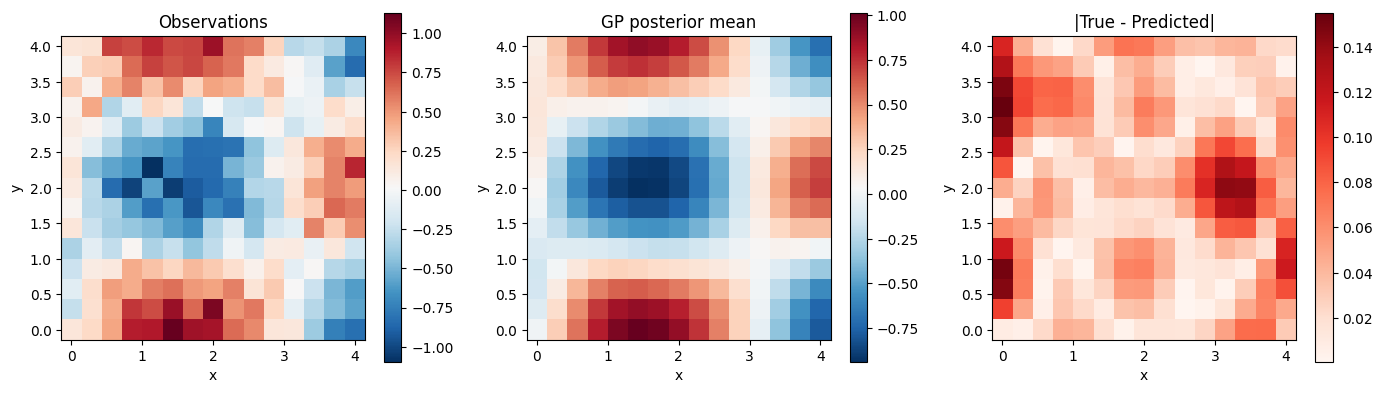

Kronecker-only operations¶

Even though we fell back to dense for the noisy solve, the Kronecker structure enables cheap operations on the kernel itself.

print("logdet(Kx kron Ky):")
print(f"  Structured: {gaussx.logdet(K_kron):.4f}")
print(f"  Dense:      {jnp.linalg.slogdet(K_kron.as_matrix())[1]:.4f}")

print("\ntrace(Kx kron Ky):")
print(f"  Structured: {gaussx.trace(K_kron):.4f}")
print(f"  Dense:      {jnp.trace(K_kron.as_matrix()):.4f}")

L_kron = gaussx.cholesky(K_kron)
print(f"\ncholesky type: {type(L_kron).__name__}")

logdet(Kx kron Ky):

  Structured: -4064.3464
  Dense:      -3904.5906

trace(Kx kron Ky):
  Structured: 225.0000

  Dense:      225.0000

cholesky type: Kronecker

References¶

Gilboa, E., Saatci, Y., & Cunningham, J. P. (2015). Scaling multidimensional inference for structured Gaussian processes. IEEE TPAMI, 37(2), 424--436.
Rasmussen, C. E. & Williams, C. K. I. (2006). Gaussian Processes for Machine Learning. MIT Press.
Saatci, Y. (2012). Scalable Inference for Structured Gaussian Process Models. PhD thesis, University of Cambridge.