Catalog — build → query → load (intro)

Catalog intro — build → query → load on a real Sentinel-2 archive¶

This notebook walks the canonical geocatalog flow against a real Sentinel-2 L2A archive over Lake Tahoe — eight scenes spanning June 2024 pulled from Microsoft Planetary Computer. We:

Discover items via STAC, sign their asset URLs.
Build a GeoCatalog from the signed URLs (one row per scene).
Run spatial + temporal queries.
Mosaic and time-stack matching rows into GeoTensors.

No synthetic GeoTIFFs, no tempfile setup — the catalog flow is the only substrate, and the URLs are real.

import json

import geocatalog as gc
import matplotlib.pyplot as plt
import numpy as np
import pandas as pd
from geostack import LAKE_TAHOE_BBOX, LAKE_TAHOE_TILE, load_stac_items

1. Discover scenes via STAC¶

Eight cloud-free Sentinel-2 L2A items over Lake Tahoe in June 2024 — load_stac_items does the search + signing.

items = load_stac_items(
    "sentinel-2-l2a",
    LAKE_TAHOE_BBOX,
    "2024-06-01/2024-07-31",
    tile=LAKE_TAHOE_TILE,
    max_cloud_cover=15,
)
print(f"found {len(items)} S2 L2A items on MGRS tile {LAKE_TAHOE_TILE}")
for it in items[:5]:
    print(f"  {it.id}  cloud_cover={it.properties['eo:cloud_cover']:.2f}%")

found 22 S2 L2A items on MGRS tile 10SGJ
  S2A_MSIL2A_20240729T183921_R070_T10SGJ_20240730T023050  cloud_cover=0.00%
  S2B_MSIL2A_20240614T183919_R070_T10SGJ_20240615T003207  cloud_cover=0.01%
  S2A_MSIL2A_20240709T183921_R070_T10SGJ_20240710T024627  cloud_cover=0.01%
  S2A_MSIL2A_20240629T183921_R070_T10SGJ_20240630T032941  cloud_cover=0.01%
  S2B_MSIL2A_20240604T183919_R070_T10SGJ_20240604T233744  cloud_cover=0.02%

2. Build a raster catalog from the signed URLs¶

build_raster_catalog reads each file’s bounds (via rasterio — /vsicurl/ for remote URLs) and a date from the filename via the (?P<date>…) named group. Sentinel-2 product IDs follow the pattern S2X_MSIL2A_YYYYMMDDTHHMMSS_… — we extract the YYYYMMDD chunk.

# One asset per scene — pick B04 (Red, 10 m). The catalog stores the
# URL + the metadata; we'll pull pixel data lazily on `load_raster`.
urls = [it.assets["B04"].href for it in items]

catalog = gc.build_raster_catalog(
    urls,
    filename_regex=r".*_(?P<date>\d{8})T\d{6}_.*\.tif",
    target_crs="EPSG:32610",
)
print(f"len(catalog): {len(catalog)}")
print(f"catalog.backend: {catalog.backend!r}")
print(f"catalog.total_bounds: {tuple(round(x, 1) for x in catalog.total_bounds)}")
print(f"catalog.temporal_extent: {catalog.temporal_extent}")

len(catalog): 22
catalog.backend: 'raster'
catalog.total_bounds: (699960.0, 4290240.0, 809760.0, 4400040.0)
catalog.temporal_extent: [2024-06-02 00:00:00, 2024-07-29 23:59:59.999999]

Inspect the underlying GeoDataFrame — one row per scene with a geometry column (footprint polygon) and an IntervalIndex row index carrying the time interval.

catalog.gdf[["filepath", "start_time", "end_time"]].head()

3. Query¶

Build a GeoSlice over the western shore of Lake Tahoe for the first week of June. Ask the catalog which rows intersect.

# UTM 10N coordinates for the Lake Tahoe AOI:
aoi_bounds_utm = (752000.0, 4320000.0, 760000.0, 4330000.0)
aoi_week1 = gc.GeoSlice(
    bounds=aoi_bounds_utm,
    interval=pd.Interval(
        pd.Timestamp("2024-06-01"), pd.Timestamp("2024-06-07"), closed="both"
    ),
    resolution=(10.0, 10.0),
    crs="EPSG:32610",
)
hits = catalog.query(aoi_week1)
print(f"first-week hits: {len(hits)}")
print(hits.gdf[["start_time", "filepath"]].to_string())

first-week hits: 3
                                                  start_time                                                                                                                                                                                                                                                                                                                                                                                                                                                                                                                                             filepath
datetime                                                                                                                                                                                                                                                                                                                                                                                                                                                                                                                                                                                                         
[2024-06-04 00:00:00, 2024-06-04 23:59:59.999999] 2024-06-04  https://sentinel2l2a01.blob.core.windows.net/sentinel2-l2/10/S/GJ/2024/06/04/S2B_MSIL2A_20240604T183919_N0510_R070_T10SGJ_20240604T233744.SAFE/GRANULE/L2A_T10SGJ_A037848_20240604T185042/IMG_DATA/R10m/T10SGJ_20240604T183919_B04_10m.tif?st=2026-05-25T14%3A11%3A18Z&se=2026-05-26T14%3A56%3A18Z&sp=rl&sv=2025-07-05&sr=c&skoid=9c8ff44a-6a2c-4dfb-b298-1c9212f64d9a&sktid=72f988bf-86f1-41af-91ab-2d7cd011db47&skt=2026-05-26T10%3A36%3A29Z&ske=2026-06-02T10%3A36%3A29Z&sks=b&skv=2025-07-05&sig=8kjQCo2Nd32T7uTnppbDEH5pCgxEL7pq1YqAFpTPEqs%3D
[2024-06-07 00:00:00, 2024-06-07 23:59:59.999999] 2024-06-07  https://sentinel2l2a01.blob.core.windows.net/sentinel2-l2/10/S/GJ/2024/06/07/S2B_MSIL2A_20240607T184919_N0510_R113_T10SGJ_20240608T003436.SAFE/GRANULE/L2A_T10SGJ_A037891_20240607T185839/IMG_DATA/R10m/T10SGJ_20240607T184919_B04_10m.tif?st=2026-05-25T14%3A11%3A18Z&se=2026-05-26T14%3A56%3A18Z&sp=rl&sv=2025-07-05&sr=c&skoid=9c8ff44a-6a2c-4dfb-b298-1c9212f64d9a&sktid=72f988bf-86f1-41af-91ab-2d7cd011db47&skt=2026-05-26T10%3A36%3A29Z&ske=2026-06-02T10%3A36%3A29Z&sks=b&skv=2025-07-05&sig=8kjQCo2Nd32T7uTnppbDEH5pCgxEL7pq1YqAFpTPEqs%3D
[2024-06-02 00:00:00, 2024-06-02 23:59:59.999999] 2024-06-02  https://sentinel2l2a01.blob.core.windows.net/sentinel2-l2/10/S/GJ/2024/06/02/S2A_MSIL2A_20240602T184921_N0510_R113_T10SGJ_20240603T032329.SAFE/GRANULE/L2A_T10SGJ_A046728_20240602T185554/IMG_DATA/R10m/T10SGJ_20240602T184921_B04_10m.tif?st=2026-05-25T14%3A11%3A18Z&se=2026-05-26T14%3A56%3A18Z&sp=rl&sv=2025-07-05&sr=c&skoid=9c8ff44a-6a2c-4dfb-b298-1c9212f64d9a&sktid=72f988bf-86f1-41af-91ab-2d7cd011db47&skt=2026-05-26T10%3A36%3A29Z&ske=2026-06-02T10%3A36%3A29Z&sks=b&skv=2025-07-05&sig=8kjQCo2Nd32T7uTnppbDEH5pCgxEL7pq1YqAFpTPEqs%3D

Cross-CRS query¶

Same query but with the AOI specified in EPSG:4326. The catalog reprojects the bbox internally — silent empty-result bugs from CRS mismatches are caught at the boundary.

aoi_4326 = gc.GeoSlice(
    bounds=LAKE_TAHOE_BBOX,
    interval=aoi_week1.interval,
    resolution=(0.0001, 0.0001),
    crs="EPSG:4326",
)
hits_4326 = catalog.query(aoi_4326)
print(f"same query via EPSG:4326: {len(hits_4326)} hits")

same query via EPSG:4326: 3 hits

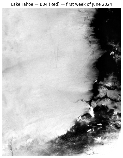
4. Load a single-scene mosaic¶

load_raster mosaics every catalog row that intersects the slice into one GeoTensor. With one row, this is a windowed read; with multiple, the merge is controlled by merge_method.

mosaic_week1 = gc.load_raster(catalog, aoi_week1, merge_method="last")
print(f"mosaic shape: {mosaic_week1.values.shape}  dtype={mosaic_week1.values.dtype}")
print(f"mosaic crs:   {mosaic_week1.crs}")

fig, ax = plt.subplots(figsize=(7, 8))
arr = mosaic_week1.values.squeeze()
ax.imshow(arr, cmap="Greys_r", vmin=np.percentile(arr, 2), vmax=np.percentile(arr, 98))
ax.set_title("Lake Tahoe — B04 (Red) — first week of June 2024")
ax.axis("off")
plt.show()

mosaic shape: (1, 1000, 800)  dtype=uint16
mosaic crs:   EPSG:32610

5. Time-series stacking¶

load_raster_timeseries walks the catalog day by day and stacks the daily mosaics along a leading time axis. Over the full eight-week AOI we get one B04 mosaic per acquisition date.

aoi_full = gc.GeoSlice(
    bounds=aoi_bounds_utm,
    interval=pd.Interval(
        pd.Timestamp("2024-06-01"), pd.Timestamp("2024-07-31"), closed="both"
    ),
    resolution=(10.0, 10.0),
    crs="EPSG:32610",
)
series = gc.load_raster_timeseries(catalog, aoi_full)
print(f"time-series shape: {series.values.shape}")
print(f"  T = {series.values.shape[0]} distinct acquisition dates")

T = series.values.shape[0]
fig, axes = plt.subplots(1, T, figsize=(2.6 * T, 3.5))
for i, ax in enumerate(np.atleast_1d(axes)):
    arr = series.values[i].squeeze()
    ax.imshow(
        arr,
        cmap="Greys_r",
        vmin=np.percentile(arr, 2),
        vmax=np.percentile(arr, 98),
    )
    ax.set_title(f"t={i}", fontsize=9)
    ax.set_xticks([])
    ax.set_yticks([])
plt.suptitle("Per-date B04 mosaics over Lake Tahoe (June–July 2024)")
plt.tight_layout()
plt.show()

time-series shape: (22, 1, 1000, 800)
  T = 22 distinct acquisition dates

6. `get_config()`¶

Every catalog returns a JSON-serialisable summary — handy for logging and reproducibility audits.

print(json.dumps(catalog.get_config(), indent=2))

{
  "backend": "raster",
  "len": 22,
  "crs": "EPSG:32610"
}

Where next¶

02_backends — raster (here), xarray, and vector catalog backends on heterogeneous real data.
03_set_algebra — query / intersect / union over multiple real catalogs.
04_duckdb — DuckDBGeoCatalog against the Overture buildings GeoParquet (billions of rows).
05_patching_bridge — CatalogDomain plugs the catalog into the same SpatialPatcher pipeline from the patching deep dives.