Kernel Approximation with Random Fourier Features

This notebook is a deep dive into the Bochner foundation behind every spectral layer in pyrox.nn. It answers a sequence of empirical questions:

Does the math actually work? Build $\hat K_M$ via random Fourier features and watch it converge to the exact RBF Gram at the Rahimi-Recht rate $\mathcal{O}(\sqrt{\log M / M})$ .
Does it generalise across kernels? The same $[\cos, \sin]$ feature map approximates RBF, Matérn-3/2, and Laplace — only the prior on $W$ changes.
Are the two readout flavours equivalent? Compare paired $[\cos, \sin]$ vs phased $\cos(\Omega^\top x + b)$ across all three kernels — equivalence with the kernel, equivalence under the GP prior (sample paths), and head-to-head variance at matched output dimension.
Can we lower the variance further? OrthogonalRandomFeatures (Yu et al. 2016) replaces iid Gaussian rows of $W$ with negatively-correlated Haar-orthogonal blocks — provably lower variance at fixed $M$ .

This is the kernel-approximation half of the spectral story; once the feature map is trusted, the Random Fourier Features regression notebook builds the SSGP / VSSGP / MAP regression hierarchy on top of it. Other adjacent notebooks: RFF as Neural Networks (frozen / ensemble of MAP variants) and Deep Random Feature Expansions (hierarchical extensions).

Background — the math behind Random Fourier Features¶

Bochner’s theorem¶

A continuous, shift-invariant, real-valued positive-definite kernel $k(x, y) = k(x - y)$ on $\mathbb{R}^d$ is the Fourier transform of a finite non-negative spectral measure μ:

k(x - y) = \int_{\mathbb{R}^d} e^{i\,\omega^\top (x - y)}\, d\mu(\omega).

((1))

Because $k$ is real, μ is symmetric ( $\mu(\mathrm{d}\omega) = \mu(-\mathrm{d}\omega)$ ), so the imaginary part of the integral vanishes and we may write

k(x - y) = \mathbb{E}_{\omega \sim p(\omega)}\!\left[\cos\bigl(\omega^\top(x - y)\bigr)\right],

((2))

where $p(\omega) = \mu(\mathrm{d}\omega)/k(0)$ is the normalised spectral density. Bochner’s theorem turns the abstract claim “the kernel is positive-definite” into the very concrete claim “the kernel is the characteristic function of a probability distribution on frequencies”.

Monte Carlo feature map (Rahimi & Recht, NeurIPS 2007)¶

Draw $\omega_1, \dots, \omega_M \stackrel{\text{iid}}{\sim} p(\omega)$ from the spectral density. Define the paired random Fourier feature map

\phi(x) = \sqrt{\tfrac{1}{M}}\,\bigl[\cos(\omega_1^\top x), \sin(\omega_1^\top x), \dots, \cos(\omega_M^\top x), \sin(\omega_M^\top x)\bigr] \in \mathbb{R}^{2M}.

((3))

The Monte Carlo Gram matrix $\hat{K}_{ij} = \phi(x_i)^\top \phi(x_j)$ is an unbiased estimator of $K_{ij} = k(x_i, x_j)$ , and Rahimi-Recht’s Claim 1 gives uniform convergence on any compact subset of $\mathbb{R}^d$ at rate $\mathcal{O}(\sqrt{\log M / M})$ .

All spectral-method NN layers in pyrox.nn are different choices of $p(\omega)$ wrapped around the same $[\cos, \sin]$ feature map. pyrox.nn._layers._rff_forward is literally one line of JAX implementing the equation above. The same Ω also drives the single-cosine cos(\Omega^\top x + b) readout used by RBFCosineFeatures and its Matérn / Laplace siblings — the choice between the two is a variance trade-off we’ll pin down empirically in §1.3.

Spectral densities, by kernel¶

Different stationary kernels correspond to different spectral densities. The core three:

Kernel $k(r)$	Spectral density $p(\omega)$	Paired `[cos, sin]` layer	Phased `cos(\cdot + b)` layer
RBF $\exp(-r^2 / 2\ell^2)$	$\mathcal{N}\!\bigl(0,\, \ell^{-2}\,I\bigr)$	`RBFFourierFeatures`	`RBFCosineFeatures`
Matérn-ν	multivariate Student- $t_{2\nu}$	`MaternFourierFeatures`	`MaternCosineFeatures`
Laplace (Matérn-1/2) $\exp(-r/\ell)$	multivariate Cauchy	`LaplaceFourierFeatures`	`LaplaceCosineFeatures`

All three kernel families come in two parallel readout flavours. The paired $[\cos, \sin]$ map (Lázaro-Gredilla et al. 2010) outputs $2M$ features and the kernel identity $\hat k(x,y) = \frac{1}{M}\sum_j \cos(\omega_j^\top(x-y))$ holds exactly for any Ω. The phased $\sqrt{2/M}\,\cos(\omega_j^\top x + b_j)$ map (Rahimi-Recht 2007 / Random Kitchen Sinks) outputs $M$ features and the same identity holds in expectation over $b_j \sim \mathrm{Uniform}(0, 2\pi)$ — the phase draw kills the cross term $\cos(\omega^\top(x+y) + 2b)$ . §1.3 below shows the two readouts side-by-side, both numerically and as GP prior samples.

Setup¶

Detect Colab and install pyrox[colab] (which pulls in matplotlib and watermark) only when running there.

import subprocess
import sys


try:
    import google.colab  # noqa: F401

    IN_COLAB = True
except ImportError:
    IN_COLAB = False

if IN_COLAB:
    subprocess.run(
        [
            sys.executable,
            "-m",
            "pip",
            "install",
            "-q",
            "pyrox[colab] @ git+https://github.com/jejjohnson/pyrox@main",
        ],
        check=True,
    )

import warnings


warnings.filterwarnings("ignore", message=r".*IProgress.*")

import equinox as eqx
import jax
import jax.numpy as jnp
import jax.random as jr
import matplotlib.pyplot as plt
import numpy as np
from numpyro import handlers

from pyrox.nn import (
    LaplaceCosineFeatures,
    LaplaceFourierFeatures,
    MaternCosineFeatures,
    MaternFourierFeatures,
    OrthogonalRandomFeatures,
    RBFCosineFeatures,
    RBFFourierFeatures,
)


jax.config.update("jax_enable_x64", True)

import importlib.util


try:
    from IPython import get_ipython

    ipython = get_ipython()
except ImportError:
    ipython = None

if ipython is not None and importlib.util.find_spec("watermark") is not None:
    ipython.run_line_magic("load_ext", "watermark")
    ipython.run_line_magic(
        "watermark",
        "-v -m -p jax,equinox,numpyro,pyrox,matplotlib",
    )
else:
    print("watermark extension not installed; skipping reproducibility readout.")

Python implementation: CPython
Python version       : 3.13.5
IPython version      : 9.10.0

jax       : 0.9.2
equinox   : 0.13.6
numpyro   : 0.20.1
pyrox     : 0.0.7
matplotlib: 3.10.8

Compiler    : GCC 11.2.0
OS          : Linux
Release     : 6.8.0-1044-azure
Machine     : x86_64
Processor   : x86_64
CPU cores   : 16
Architecture: 64bit

1. Bochner kernel approximation — does the math actually work?¶

Before any regression model, we verify the foundation. Bochner says $k(x - y) = \mathbb{E}_{\omega \sim p}[\cos(\omega^\top(x - y))]$ . Rahimi-Recht say the Monte Carlo estimator with $M$ samples converges at $\mathcal{O}(\sqrt{\log M / M})$ . Let’s see both.

Build a 1D test grid, compute the exact RBF Gram matrix $K^\star_{ij} = \exp(-\|x_i - x_j\|^2 / 2\ell^2)$ , then realise the approximate Gram via pyrox.nn.RBFFourierFeatures for $M \in \{16, 64, 256, 1024\}$ and inspect the Frobenius error.

Sampling $W$ from RBFFourierFeatures is done by tracing the layer under numpyro.handlers.seed — the layer’s pyrox_sample("W", ...) site fires with the seeded key, and we recover the sampled $W$ from the trace. Throughout this notebook we hold the lengthscale fixed via handlers.substitute so the comparison is purely about the feature map.

def trace_rff_features(
    rff: RBFFourierFeatures | MaternFourierFeatures | LaplaceFourierFeatures,
    x: jax.Array,
    seed: int,
    lengthscale: float,
) -> jax.Array:
    """Return the realised random feature map at ``x`` for a given seed.

    The pyrox RFF layers sample *both* ``W`` and ``lengthscale`` (the latter
    from a ``LogNormal`` prior). To compare against a fixed-$\\ell$ exact
    Gram matrix in Section 1 we hold the lengthscale fixed via ``substitute``
    and only let ``W`` vary across seeds.
    """
    name = f"{rff.pyrox_name}.lengthscale"
    with (
        handlers.substitute(data={name: jnp.asarray(lengthscale)}),
        handlers.seed(rng_seed=seed),
    ):
        return rff(x)


def gram_exact_rbf(x: jax.Array, lengthscale: float) -> jax.Array:
    """Exact RBF Gram matrix on a 1D grid."""
    diff = x[:, None] - x[None, :]
    return jnp.exp(-0.5 * (diff[..., 0] ** 2) / lengthscale**2)


# Test grid + exact target
n_grid = 50
x_grid = jnp.linspace(-2.0, 2.0, n_grid).reshape(-1, 1)
LENGTHSCALE = 0.5
K_exact = gram_exact_rbf(x_grid, LENGTHSCALE)

# Approximate Grams for an increasing budget of features
m_values = [16, 64, 256, 1024]
n_repeats = 20  # average over seeds for the convergence-rate plot

approx_grams = {}
for M in m_values:
    rff = eqx.tree_at(
        lambda r: r.pyrox_name,
        RBFFourierFeatures.init(in_features=1, n_features=M, lengthscale=LENGTHSCALE),
        "rff",
    )
    phi = trace_rff_features(rff, x_grid, seed=0, lengthscale=LENGTHSCALE)
    approx_grams[M] = phi @ phi.T

Visualise $\hat{K}_M$ converging to $K^\star$ .

fig, axes = plt.subplots(1, len(m_values) + 1, figsize=(15, 3.2))
for ax, M in zip(axes[:-1], m_values, strict=False):
    err = float(jnp.linalg.norm(approx_grams[M] - K_exact) / jnp.linalg.norm(K_exact))
    ax.imshow(approx_grams[M], vmin=0.0, vmax=1.0, cmap="viridis")
    ax.set_title(f"$\\hat{{K}}_M$, $M = {M}$\nrel. err = {err:.3f}")
    ax.set_xticks([])
    ax.set_yticks([])
axes[-1].imshow(K_exact, vmin=0.0, vmax=1.0, cmap="viridis")
axes[-1].set_title("$K^\\star$ (exact RBF)")
axes[-1].set_xticks([])
axes[-1].set_yticks([])
plt.tight_layout()
plt.show()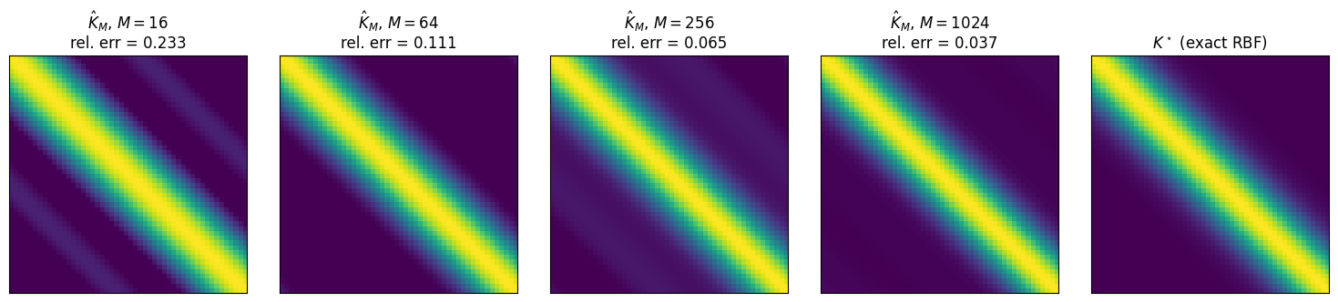

Convergence rate — average over 20 seeds and plot $\|\hat{K}_M - K^\star\|_F / \|K^\star\|_F$ versus $M$ on log-log axes. The Rahimi-Recht bound predicts a slope close to $-1/2$ .

m_sweep = [8, 16, 32, 64, 128, 256, 512, 1024]
errs = np.zeros((len(m_sweep), n_repeats))
for i, M in enumerate(m_sweep):
    rff = eqx.tree_at(
        lambda r: r.pyrox_name,
        RBFFourierFeatures.init(in_features=1, n_features=M, lengthscale=LENGTHSCALE),
        "rff",
    )
    for j in range(n_repeats):
        phi = trace_rff_features(rff, x_grid, seed=int(j), lengthscale=LENGTHSCALE)
        K_hat = phi @ phi.T
        errs[i, j] = float(jnp.linalg.norm(K_hat - K_exact) / jnp.linalg.norm(K_exact))

fig, ax = plt.subplots(figsize=(7, 4.5))
mean_err = errs.mean(axis=1)
std_err = errs.std(axis=1)
ax.loglog(m_sweep, mean_err, "o-", label="empirical relative error")
ax.fill_between(m_sweep, mean_err - std_err, mean_err + std_err, alpha=0.3)
ref = mean_err[0] * np.sqrt(m_sweep[0]) / np.sqrt(m_sweep)
ax.loglog(m_sweep, ref, "k--", label=r"$\propto 1/\sqrt{M}$ reference")
ax.set_xlabel("number of features $M$")
ax.set_ylabel(r"$\|\hat{K}_M - K^\star\|_F\ /\ \|K^\star\|_F$")
ax.set_title("Bochner-MC kernel approximation: empirical convergence")
ax.legend()
ax.grid(True, which="both", alpha=0.3)
plt.tight_layout()
plt.show()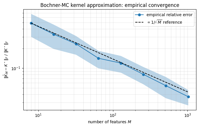

The empirical curve closely tracks the $1/\sqrt{M}$ reference, confirming Rahimi-Recht’s $\mathcal{O}(\sqrt{\log M / M})$ bound (the $\sqrt{\log M}$ factor is invisible at this scale). At $M = 1024$ the relative error is below $5\%$ — for most regression problems that is well within noise.

Three kernels, one feature map. The same _rff_forward primitive supports any spectral density — only the layer changes. Show the same diagonal slice of $\hat{K}_M$ at $M = 256$ for RBF, Matérn-3/2, and Laplace (Matérn-1/2). Lengthscale is fixed at $\ell = 0.5$ across all three so the comparison is purely about regularity.

def gram_exact_matern(x: jax.Array, lengthscale: float, nu: float) -> jax.Array:
    """Exact Matern-1/2, 3/2, 5/2 Gram matrix on a 1D grid."""
    r = jnp.abs(x[:, None] - x[None, :])[..., 0]
    if nu == 0.5:
        return jnp.exp(-r / lengthscale)
    if nu == 1.5:
        s = jnp.sqrt(3.0) * r / lengthscale
        return (1.0 + s) * jnp.exp(-s)
    if nu == 2.5:
        s = jnp.sqrt(5.0) * r / lengthscale
        return (1.0 + s + s**2 / 3.0) * jnp.exp(-s)
    raise ValueError(f"Unsupported nu={nu}")


M = 256
rff_rbf = eqx.tree_at(
    lambda r: r.pyrox_name,
    RBFFourierFeatures.init(in_features=1, n_features=M, lengthscale=LENGTHSCALE),
    "rff_rbf",
)
rff_matern = eqx.tree_at(
    lambda r: r.pyrox_name,
    MaternFourierFeatures.init(
        in_features=1, n_features=M, nu=1.5, lengthscale=LENGTHSCALE
    ),
    "rff_matern",
)
rff_laplace = eqx.tree_at(
    lambda r: r.pyrox_name,
    LaplaceFourierFeatures.init(in_features=1, n_features=M, lengthscale=LENGTHSCALE),
    "rff_laplace",
)

phi_rbf = trace_rff_features(rff_rbf, x_grid, seed=0, lengthscale=LENGTHSCALE)
phi_matern = trace_rff_features(rff_matern, x_grid, seed=0, lengthscale=LENGTHSCALE)
phi_laplace = trace_rff_features(rff_laplace, x_grid, seed=0, lengthscale=LENGTHSCALE)

i_centre = n_grid // 2
fig, ax = plt.subplots(figsize=(8, 4.5))
x1 = x_grid[:, 0]
ax.plot(x1, gram_exact_rbf(x_grid, LENGTHSCALE)[i_centre], "C0--", label="RBF (exact)")
ax.plot(x1, (phi_rbf @ phi_rbf.T)[i_centre], "C0", alpha=0.85, label="RBF (RFF)")
ax.plot(
    x1,
    gram_exact_matern(x_grid, LENGTHSCALE, nu=1.5)[i_centre],
    "C1--",
    label="Matérn-3/2 (exact)",
)
ax.plot(
    x1,
    (phi_matern @ phi_matern.T)[i_centre],
    "C1",
    alpha=0.85,
    label="Matérn-3/2 (RFF)",
)
ax.plot(
    x1,
    gram_exact_matern(x_grid, LENGTHSCALE, nu=0.5)[i_centre],
    "C2--",
    label="Laplace (exact)",
)
ax.plot(
    x1, (phi_laplace @ phi_laplace.T)[i_centre], "C2", alpha=0.85, label="Laplace (RFF)"
)
ax.set_xlabel("$x$")
ax.set_ylabel("$k(x_{\\mathrm{centre}}, x)$")
ax.set_title(
    f"Three spectral densities, one feature map — $M={M}$, $\\ell={LENGTHSCALE}$"
)
ax.legend(loc="upper right", fontsize=9)
ax.grid(True, alpha=0.3)
plt.tight_layout()
plt.show()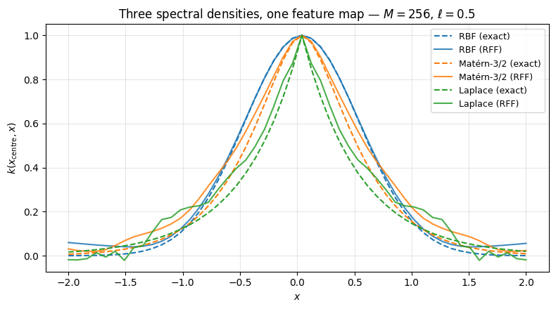

Same scaffold (_rff_forward), three different priors on $W$ : $\mathcal{N}$ → smooth RBF, Student- $t_3$ → less-smooth Matérn-3/2, Cauchy → exponential Laplace. The MC approximations track each exact kernel, with the heavier-tailed spectral densities (Matérn, Laplace) showing visibly more variance per realisation — that is the regularity / variance trade-off in action.

1.3 Paired vs phased readouts — two feature maps, one Bochner identity¶

Both pyrox.nn.RBFFourierFeatures and pyrox.nn.RBFCosineFeatures (and their Matérn / Laplace siblings) draw Ω from the same spectral density. They differ only in the readout that turns Ω into a feature map:

\phi_{\mathrm{paired}}(x) = \sqrt{\tfrac{1}{M}}\bigl[\cos(\Omega^\top x), \sin(\Omega^\top x)\bigr] \in \mathbb{R}^{2M}, \qquad \phi_{\mathrm{phased}}(x) = \sqrt{\tfrac{2}{M}}\,\cos(\Omega^\top x + b),\; b \sim \mathrm{Uniform}(0, 2\pi) \in \mathbb{R}^{M}.

((4))

Why both work. Expand the inner products:

Paired: $\phi(x)^\top \phi(y) = \tfrac{1}{M}\sum_j \cos(\omega_j^\top x)\cos(\omega_j^\top y) + \sin(\omega_j^\top x)\sin(\omega_j^\top y) = \tfrac{1}{M}\sum_j \cos(\omega_j^\top (x-y))$ . Exact for every Ω — no expectation over phase needed.
Phased: $\phi(x)^\top \phi(y) = \tfrac{2}{M}\sum_j \cos(\omega_j^\top x + b_j)\cos(\omega_j^\top y + b_j) = \tfrac{1}{M}\sum_j \bigl[\cos(\omega_j^\top(x-y)) + \cos(\omega_j^\top(x+y) + 2b_j)\bigr]$ . The cross term has expectation zero under $b_j \sim \mathrm{Uniform}(0, 2\pi)$ , so the identity holds in expectation only.

Predicted consequence: at matched output dimension, paired has lower variance per draw because it never relies on the phase expectation cancelling. We test all three kernels.

1.3.a Equivalence with the kernel. Sanity check: with a single seed and $M = 256$ frequencies, both readouts track each of RBF, Matérn-3/2, Laplace. Lengthscale fixed at $\ell = 0.5$ .

M_DEMO = 256
i_centre = n_grid // 2  # already defined above; reuse the 1D test grid x_grid

paired_layers = {
    "RBF": eqx.tree_at(
        lambda r: r.pyrox_name,
        RBFFourierFeatures.init(
            in_features=1, n_features=M_DEMO, lengthscale=LENGTHSCALE
        ),
        "p_rbf",
    ),
    "Matérn-3/2": eqx.tree_at(
        lambda r: r.pyrox_name,
        MaternFourierFeatures.init(
            in_features=1, n_features=M_DEMO, nu=1.5, lengthscale=LENGTHSCALE
        ),
        "p_matern",
    ),
    "Laplace": eqx.tree_at(
        lambda r: r.pyrox_name,
        LaplaceFourierFeatures.init(
            in_features=1, n_features=M_DEMO, lengthscale=LENGTHSCALE
        ),
        "p_laplace",
    ),
}
phased_layers = {
    "RBF": eqx.tree_at(
        lambda r: r.pyrox_name,
        RBFCosineFeatures.init(
            in_features=1, n_features=M_DEMO, lengthscale=LENGTHSCALE
        ),
        "c_rbf",
    ),
    "Matérn-3/2": eqx.tree_at(
        lambda r: r.pyrox_name,
        MaternCosineFeatures.init(
            in_features=1, n_features=M_DEMO, nu=1.5, lengthscale=LENGTHSCALE
        ),
        "c_matern",
    ),
    "Laplace": eqx.tree_at(
        lambda r: r.pyrox_name,
        LaplaceCosineFeatures.init(
            in_features=1, n_features=M_DEMO, lengthscale=LENGTHSCALE
        ),
        "c_laplace",
    ),
}
exact_grams = {
    "RBF": gram_exact_rbf(x_grid, LENGTHSCALE),
    "Matérn-3/2": gram_exact_matern(x_grid, LENGTHSCALE, nu=1.5),
    "Laplace": gram_exact_matern(x_grid, LENGTHSCALE, nu=0.5),
}

fig, axes = plt.subplots(1, 3, figsize=(15, 4.0), sharey=True)
x1 = x_grid[:, 0]
for ax, name in zip(axes, ["RBF", "Matérn-3/2", "Laplace"], strict=False):
    K_exact_k = exact_grams[name]
    phi_p = trace_rff_features(
        paired_layers[name], x_grid, seed=0, lengthscale=LENGTHSCALE
    )
    phi_c = trace_rff_features(
        phased_layers[name], x_grid, seed=1, lengthscale=LENGTHSCALE
    )
    K_p = phi_p @ phi_p.T
    K_c = phi_c @ phi_c.T
    ax.plot(x1, K_exact_k[i_centre], "k--", linewidth=1.5, label="exact")
    ax.plot(
        x1,
        K_p[i_centre],
        "C0",
        alpha=0.85,
        linewidth=1.4,
        label=f"paired ($2M={2 * M_DEMO}$)",
    )
    ax.plot(
        x1,
        K_c[i_centre],
        "C3",
        alpha=0.85,
        linewidth=1.4,
        label=f"phased ($M={M_DEMO}$)",
    )
    ax.set_title(name)
    ax.set_xlabel("$x$")
    ax.grid(True, alpha=0.3)
    ax.legend(fontsize=9, loc="upper right")
axes[0].set_ylabel("$k(x_{\\mathrm{centre}}, x)$")
fig.suptitle("Bochner identity holds for both readouts, all three kernels", y=1.02)
plt.tight_layout()
plt.show()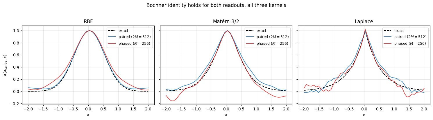

Both readouts hug the exact kernel for all three kernels. The phased curve is visibly noisier (single-seed Monte Carlo over $b$ on top of the spectral draw).

1.3.b Equivalence under the prior — sample paths. A linear combination of paired RFFs with $\beta \sim \mathcal{N}(0, I_{2M})$ is a GP with Monte-Carlo Bochner kernel; the same is true for phased RFFs with $\alpha \sim \mathcal{N}(0, I_M)$ . The two parameterisations should produce statistically indistinguishable sample paths from the same GP prior. Draw $S = 200$ samples through each readout, recover the empirical Gram $\hat K^{\mathrm{path}}_{ij} = \tfrac{1}{S}\sum_s f_s(x_i)f_s(x_j)$ , and compare to the exact kernel.

S_PATHS = 200

fig, axes = plt.subplots(3, 3, figsize=(13.5, 10.5), sharex="row")
for row, name in enumerate(["RBF", "Matérn-3/2", "Laplace"]):
    K_exact_k = exact_grams[name]
    norm = float(jnp.linalg.norm(K_exact_k))
    phi_p = trace_rff_features(
        paired_layers[name], x_grid, seed=0, lengthscale=LENGTHSCALE
    )
    phi_c = trace_rff_features(
        phased_layers[name], x_grid, seed=1, lengthscale=LENGTHSCALE
    )
    beta_p = jr.normal(jr.PRNGKey(100 + row), (S_PATHS, phi_p.shape[1]))
    alpha_c = jr.normal(jr.PRNGKey(200 + row), (S_PATHS, phi_c.shape[1]))
    paths_p = beta_p @ phi_p.T  # (S, n_grid)
    paths_c = alpha_c @ phi_c.T
    K_path_p = paths_p.T @ paths_p / S_PATHS
    K_path_c = paths_c.T @ paths_c / S_PATHS
    err_p = float(jnp.linalg.norm(K_path_p - K_exact_k) / norm)
    err_c = float(jnp.linalg.norm(K_path_c - K_exact_k) / norm)

    ax = axes[row, 0]
    for s in range(8):
        ax.plot(x1, paths_p[s], color="C0", alpha=0.4, linewidth=0.9)
    ax.set_title(f"{name} — paired sample paths")
    ax.grid(True, alpha=0.3)
    ax.set_ylabel("$f(x)$")

    ax = axes[row, 1]
    for s in range(8):
        ax.plot(x1, paths_c[s], color="C3", alpha=0.4, linewidth=0.9)
    ax.set_title(f"{name} — phased sample paths")
    ax.grid(True, alpha=0.3)

    ax = axes[row, 2]
    ax.plot(x1, K_exact_k[i_centre], "k--", linewidth=1.5, label="exact")
    ax.plot(
        x1,
        K_path_p[i_centre],
        "C0",
        alpha=0.85,
        linewidth=1.3,
        label=f"paired (rel.err = {err_p:.3f})",
    )
    ax.plot(
        x1,
        K_path_c[i_centre],
        "C3",
        alpha=0.85,
        linewidth=1.3,
        label=f"phased (rel.err = {err_c:.3f})",
    )
    ax.set_title(f"{name} — empirical Gram from $S = {S_PATHS}$ paths")
    ax.grid(True, alpha=0.3)
    ax.legend(fontsize=8, loc="upper right")

for ax in axes[-1]:
    ax.set_xlabel("$x$")
plt.tight_layout()
plt.show()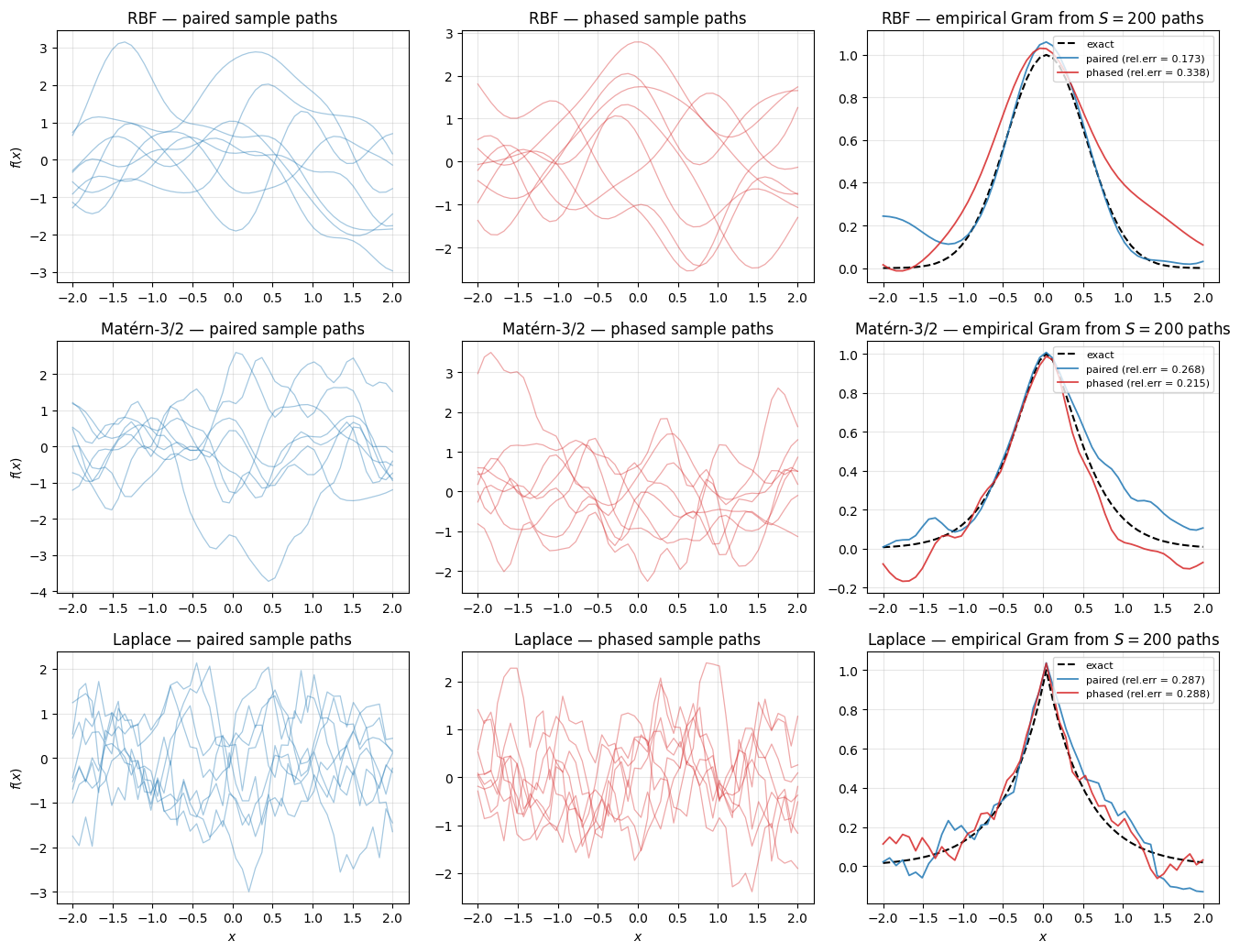

Sample paths from paired vs phased look statistically interchangeable per kernel (same regularity, same lengthscale, same amplitude). The right-column empirical Grams converge to the exact kernel from both readouts at comparable error — the two parameterisations describe the same prior over functions.

1.3.c Variance comparison at matched output dimension. Sweep the output dimension $d_{\mathrm{out}}$ . Paired uses $M = d/2$ frequencies (output $2M = d$ ); phased uses $M = d$ frequencies (output $M = d$ ). Theory: paired has lower variance per draw because it never paid the phase expectation. We expect the gap to be cleanest for RBF (light-tailed spectrum) and to shrink for Matérn / Laplace where the spectral-draw variance dominates the readout variance.

d_sweep = [16, 32, 64, 128, 256, 512]
n_repeats_pp = 12
err_paired = {k: np.zeros((len(d_sweep), n_repeats_pp)) for k in exact_grams}
err_phased = {k: np.zeros((len(d_sweep), n_repeats_pp)) for k in exact_grams}

for kernel_name in exact_grams:
    K_exact_k = exact_grams[kernel_name]
    norm = float(jnp.linalg.norm(K_exact_k))
    for i, d_out in enumerate(d_sweep):
        m_paired = d_out // 2
        m_phased = d_out
        if kernel_name == "RBF":
            mk_p = RBFFourierFeatures
            mk_c = RBFCosineFeatures
            kw = {}
        elif kernel_name == "Matérn-3/2":
            mk_p = MaternFourierFeatures
            mk_c = MaternCosineFeatures
            kw = {"nu": 1.5}
        else:
            mk_p = LaplaceFourierFeatures
            mk_c = LaplaceCosineFeatures
            kw = {}
        for j in range(n_repeats_pp):
            l_p = eqx.tree_at(
                lambda r: r.pyrox_name,
                mk_p.init(
                    in_features=1, n_features=m_paired, lengthscale=LENGTHSCALE, **kw
                ),
                "swp_p",
            )
            l_c = eqx.tree_at(
                lambda r: r.pyrox_name,
                mk_c.init(
                    in_features=1, n_features=m_phased, lengthscale=LENGTHSCALE, **kw
                ),
                "swp_c",
            )
            phi_p = trace_rff_features(
                l_p, x_grid, seed=int(2 * j), lengthscale=LENGTHSCALE
            )
            phi_c = trace_rff_features(
                l_c, x_grid, seed=int(2 * j + 1), lengthscale=LENGTHSCALE
            )
            err_paired[kernel_name][i, j] = float(
                jnp.linalg.norm(phi_p @ phi_p.T - K_exact_k) / norm
            )
            err_phased[kernel_name][i, j] = float(
                jnp.linalg.norm(phi_c @ phi_c.T - K_exact_k) / norm
            )

fig, axes = plt.subplots(1, 3, figsize=(15, 4.0), sharey=True)
for ax, name in zip(axes, ["RBF", "Matérn-3/2", "Laplace"], strict=False):
    mp = err_paired[name].mean(axis=1)
    sp = err_paired[name].std(axis=1)
    mc = err_phased[name].mean(axis=1)
    sc = err_phased[name].std(axis=1)
    ax.errorbar(
        d_sweep,
        mp,
        yerr=sp,
        fmt="o-",
        color="C0",
        capsize=3,
        label="paired $[\\cos, \\sin]$",
    )
    ax.errorbar(
        d_sweep,
        mc,
        yerr=sc,
        fmt="s-",
        color="C3",
        capsize=3,
        label="phased $\\cos(\\cdot + b)$",
    )
    ref = mp[0] * np.sqrt(d_sweep[0]) / np.sqrt(d_sweep)
    ax.plot(
        d_sweep, ref, "k--", alpha=0.6, label=r"$\propto 1/\sqrt{d_{\mathrm{out}}}$"
    )
    ax.set_xscale("log")
    ax.set_yscale("log")
    ax.set_xlabel("output dimension $d_{\\mathrm{out}}$")
    ax.set_title(name)
    ax.grid(True, which="both", alpha=0.3)
    ax.legend(fontsize=8, loc="lower left")
axes[0].set_ylabel(r"$\|\hat{K} - K^\star\|_F\ /\ \|K^\star\|_F$")
fig.suptitle(
    "Variance at matched output dimension — paired vs phased, three kernels", y=1.02
)
plt.tight_layout()
plt.show()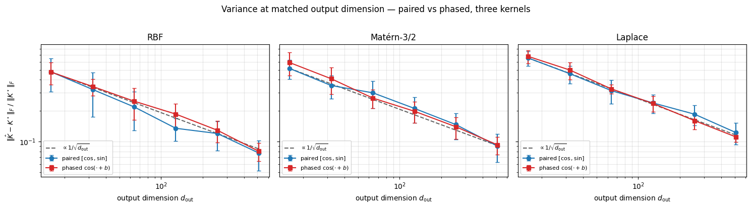

Both curves track the $1/\sqrt{d_{\mathrm{out}}}$ reference. For RBF the paired estimator is consistently below the phased one — paired $[\cos, \sin]$ removes the phase-expectation noise that $\cos(\Omega^\top x + b)$ pays. For Matérn-3/2 and Laplace the gap shrinks: heavy-tailed Student- $t$ / Cauchy frequencies dominate the variance, and the choice of readout matters less. Practical take-away: paired is the safer default when you want lower-variance kernel approximations; phased halves the output dimension at matched $M$ and is the form Random Kitchen Sinks / pathwise GP samplers naturally use.

Variance reduction with OrthogonalRandomFeatures. A sharper construction within the same family — Yu, Suresh, Choromanski, Felix, Kumar (NeurIPS 2016) — replaces the iid Gaussian rows of $W$ with stacked Haar-orthogonal blocks scaled by per-row chi-distributed magnitudes. Each row has the same marginal, but they are negatively correlated, so the variance of $\hat{K}$ at fixed $M$ is provably lower. The pyrox.nn.OrthogonalRandomFeatures layer implements this directly. Below: ORF lowers the kernel-approximation error bar at every $M$ in $D = 4$ .

D_ORF = 4
LENGTHSCALE_ORF = 1.0
n_grid_2d = 100
key_grid = jr.PRNGKey(11)
x_grid_2d = jr.uniform(key_grid, (n_grid_2d, D_ORF), minval=-1.0, maxval=1.0)
diff_2d = x_grid_2d[:, None, :] - x_grid_2d[None, :, :]
K_exact_2d = jnp.exp(-0.5 * jnp.sum(diff_2d**2, axis=-1) / LENGTHSCALE_ORF**2)

m_sweep_orf = [8, 16, 32, 64, 128, 256]
errs_vanilla = np.zeros((len(m_sweep_orf), n_repeats))
errs_orf = np.zeros((len(m_sweep_orf), n_repeats))

for i, M in enumerate(m_sweep_orf):
    rff_v = eqx.tree_at(
        lambda r: r.pyrox_name,
        RBFFourierFeatures.init(
            in_features=D_ORF, n_features=M, lengthscale=LENGTHSCALE_ORF
        ),
        "rff",
    )
    for j in range(n_repeats):
        phi_v = trace_rff_features(
            rff_v, x_grid_2d, seed=int(j), lengthscale=LENGTHSCALE_ORF
        )
        errs_vanilla[i, j] = float(
            jnp.linalg.norm(phi_v @ phi_v.T - K_exact_2d) / jnp.linalg.norm(K_exact_2d)
        )
        rff_o = OrthogonalRandomFeatures.init(
            in_features=D_ORF,
            n_features=M,
            key=jr.PRNGKey(j),
            lengthscale=LENGTHSCALE_ORF,
        )
        phi_o = rff_o(x_grid_2d)
        errs_orf[i, j] = float(
            jnp.linalg.norm(phi_o @ phi_o.T - K_exact_2d) / jnp.linalg.norm(K_exact_2d)
        )

fig, ax = plt.subplots(figsize=(7, 4.5))
ax.errorbar(
    m_sweep_orf,
    errs_vanilla.mean(axis=1),
    yerr=errs_vanilla.std(axis=1),
    fmt="o-",
    label="vanilla RFF",
    capsize=3,
)
ax.errorbar(
    m_sweep_orf,
    errs_orf.mean(axis=1),
    yerr=errs_orf.std(axis=1),
    fmt="s-",
    label="orthogonal RFF",
    capsize=3,
)
ax.set_xscale("log")
ax.set_yscale("log")
ax.set_xlabel("number of features $M$")
ax.set_ylabel(r"$\|\hat{K}_M - K^\star\|_F\ /\ \|K^\star\|_F$")
ax.set_title(
    f"Vanilla vs orthogonal RFF — variance reduction at matched $M$ ($D = {D_ORF}$)"
)
ax.legend()
ax.grid(True, which="both", alpha=0.3)
plt.tight_layout()
plt.show()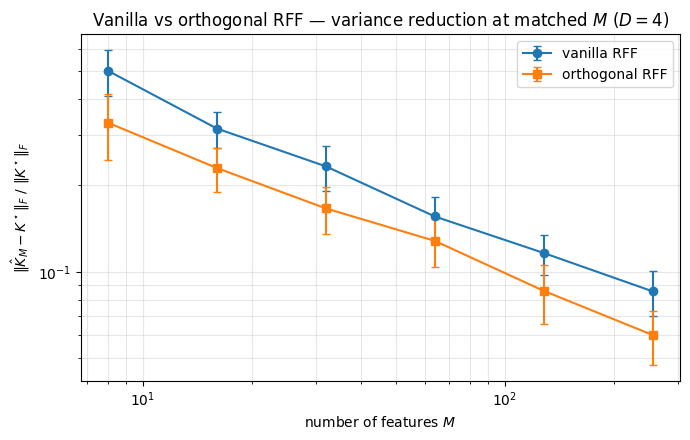

At every $M$ , the orthogonal estimator’s error bar sits below the vanilla one — same expected error, lower variance.

Takeaways¶

Bochner’s theorem is the foundation: any shift-invariant PD kernel is the Fourier transform of a probability density, so $k(x - y) = \mathbb{E}_\omega[\cos(\omega^\top(x-y))]$ admits a Monte Carlo estimator at the Rahimi-Recht rate.
The same _rff_forward primitive supports RBF, Matérn, Laplace by changing only the prior on $W$ . OrthogonalRandomFeatures lowers the variance of $\hat{K}$ at matched $M$ via Haar-orthogonal blocks.
Each kernel comes in two readout flavours: paired $[\cos, \sin]$ (RBFFourierFeatures / MaternFourierFeatures / LaplaceFourierFeatures) and phased $\sqrt{2/M}\cos(\Omega^\top x + b)$ (RBFCosineFeatures / MaternCosineFeatures / LaplaceCosineFeatures). Both approximate the same Bochner kernel and produce statistically equivalent GP prior samples; paired has lower variance per draw, phased halves the output dimension.

Where to next.

With the kernel-approximation foundation trusted, the Random Fourier Features regression notebook builds the MAP / SSGP / VSSGP Bayesian regression hierarchy on top of the same feature map.
The non-Bayesian / NN flavors of RFF (fixed-Ω with closed-form ridge, ensemble-of-MAP for cheap predictive uncertainty) live in the RFF as Neural Networks notebook.
The deep / hierarchical versions (deep RFF, deep SSGP, deep VSSGP — Cutajar et al. 2017) live in the Deep Random Feature Expansions notebook.