Random Fourier Features → SSGP → VSSGP — Three Spectral Views of a Gaussian Process

This notebook is the GP-flavored companion to the RFF as Neural Networks notebook. Where that notebook treats RFF as a neural network architecture (with frozen, learned, or ensembled weights), here we follow the Bayesian progression that links the same feature map to Gaussian processes:

Learned RFF (MAP baseline) — the deterministic regression model with trainable Ω. No uncertainty over the parameters; just a regularised MSE point estimate.
SSGP — Sparse Spectrum GP (Lázaro-Gredilla et al. JMLR 2010) — analytically marginalise the head β and train Ω on the GP marginal likelihood. Closed-form predictive variance for free.
VSSGP — Variational SSGP (Gal & Turner ICML 2015) — put a variational posterior $q(\Omega)$ on top of $q(\beta)$ , train via reparameterised ELBO. Full posterior uncertainty over both frequencies and weights.

The three are different inferential commitments to the same model class — a linear combination of $M$ random Fourier features:

y_i = \Phi(x_i; \Omega)\,\beta + \varepsilon_i, \qquad \Phi(x; \Omega) = \sqrt{\tfrac{1}{M}}\bigl[\cos(\Omega^\top x), \sin(\Omega^\top x)\bigr] \in \mathbb{R}^{2M}, \qquad \varepsilon_i \sim \mathcal{N}(0, \sigma_n^2).

((1))

Method	Ω	β	Objective	Predictive variance?
Learned RFF (MAP)	trained (point)	trained (point) + L2	regularised MSE	no
SSGP	trained (point)	marginalised analytically	log marginal likelihood	yes — closed form
VSSGP	variational $q(\Omega)$	variational $q(\beta)$	tempered ELBO	yes — MC over the posterior

Foundation. The Bochner / Rahimi-Recht derivation of the feature map, the kernel-approximation convergence rate, and the equivalence between paired $[\cos, \sin]$ and phased $\cos(\Omega^\top x + b)$ readouts across RBF / Matérn / Laplace are covered separately in the Kernel Approximation notebook. This notebook treats that map as a black box and focuses on the Bayesian inference layer.

Forward-pointers: the fixed-Ω version (Rahimi-Recht 2007) and the ensemble-of-MAP alternative live in the RFF as Neural Networks notebook. The deep versions are in the Deep Random Feature Expansions notebook.

Background — from features to GPs¶

A linear combination of $M$ random Fourier features with Gaussian weights

f(x) = \beta^\top \phi(x), \qquad \beta \sim \mathcal{N}\!\bigl(0,\, \sigma_\beta^2\,I\bigr), \qquad \phi(x) = \sqrt{\tfrac{1}{M}}\bigl[\cos(\Omega^\top x), \sin(\Omega^\top x)\bigr]

((2))

is itself a Gaussian process with kernel

\mathrm{Cov}(f(x), f(y)) = \sigma_\beta^2\,\phi(x)^\top \phi(y) = \sigma_\beta^2\,\hat{k}(x, y) \;\xrightarrow[M \to \infty]{}\; \sigma_\beta^2\,k(x, y).

((3))

This is the Sparse Spectrum GP (SSGP). The marginal likelihood and predictive distribution have closed forms — derived in §3. Per-iteration cost is $\mathcal{O}(NM^2 + M^3)$ , linear in the dataset size for fixed $M$ , the headline win over the $\mathcal{O}(N^3)$ exact GP. (For the spectral-density derivation that justifies $\hat k \to k$ — and the empirical convergence figures across RBF / Matérn / Laplace — see the Kernel Approximation notebook.)

Setup¶

Detect Colab and install pyrox[colab] (which pulls in matplotlib and watermark) only when running there.

import subprocess
import sys


try:
    import google.colab  # noqa: F401

    IN_COLAB = True
except ImportError:
    IN_COLAB = False

if IN_COLAB:
    subprocess.run(
        [
            sys.executable,
            "-m",
            "pip",
            "install",
            "-q",
            "pyrox[colab] @ git+https://github.com/jejjohnson/pyrox@main",
        ],
        check=True,
    )

import warnings


warnings.filterwarnings("ignore", message=r".*IProgress.*")

import equinox as eqx
import jax
import jax.numpy as jnp
import jax.random as jr
import matplotlib.pyplot as plt
import numpy as np
import optax


jax.config.update("jax_enable_x64", True)

import importlib.util


try:
    from IPython import get_ipython

    ipython = get_ipython()
except ImportError:
    ipython = None

if ipython is not None and importlib.util.find_spec("watermark") is not None:
    ipython.run_line_magic("load_ext", "watermark")
    ipython.run_line_magic(
        "watermark",
        "-v -m -p jax,equinox,numpyro,pyrox,matplotlib",
    )
else:
    print("watermark extension not installed; skipping reproducibility readout.")

Python implementation: CPython
Python version       : 3.13.5
IPython version      : 9.10.0

jax       : 0.9.2
equinox   : 0.13.6
numpyro   : 0.20.1
pyrox     : 0.0.7
matplotlib: 3.10.8

Compiler    : GCC 11.2.0
OS          : Linux
Release     : 6.8.0-1044-azure
Machine     : x86_64
Processor   : x86_64
CPU cores   : 16
Architecture: 64bit

Shared regression setup¶

All three regression methods (§2 learned RFF, §3 SSGP, §4 VSSGP) are evaluated on the same target with a held-out gap, so predictive uncertainty in the gap becomes the visual axis of comparison:

y_i = \sin(3\pi x_i) + 0.05\,\varepsilon_i, \qquad \varepsilon_i \sim \mathcal{N}(0, 1), \qquad x_i \in [-1, -0.2] \cup [0.4, 1].

((4))

The target frequency is $\omega^\star = 3\pi \approx 9.42$ . We use a lengthscale prior $\ell = 0.3$ throughout, giving prior frequency standard deviation $1/\ell \approx 3.3$ — comfortable coverage of $\omega^\star$ . All three methods use $M = 64$ Fourier features.

N_OBS, NOISE_STD = 80, 0.05
x_full = jnp.linspace(-1.0, 1.0, N_OBS)
mask = (x_full < -0.2) | (x_full > 0.4)
x_obs = x_full[mask].reshape(-1, 1)
y_obs = jnp.sin(3.0 * jnp.pi * x_obs[:, 0]) + NOISE_STD * jr.normal(
    jr.PRNGKey(2), x_obs.shape[0:1]
)

x_test = jnp.linspace(-1.2, 1.2, 400).reshape(-1, 1)
y_truth = jnp.sin(3.0 * jnp.pi * x_test[:, 0])

M_FEAT = 64
LENGTHSCALE_INIT = 0.3
TARGET_OMEGA = 3.0 * jnp.pi
print(f"target frequency: ω⋆ = 3π ≈ {float(TARGET_OMEGA):.2f}")
print(f"prior bandwidth at ℓ={LENGTHSCALE_INIT}: 1/ℓ ≈ {1.0 / LENGTHSCALE_INIT:.2f}")
print(f"observation count: N = {x_obs.shape[0]}, gap removed from x ∈ (-0.2, 0.4)")

target frequency: ω⋆ = 3π ≈ 9.42
prior bandwidth at ℓ=0.3: 1/ℓ ≈ 3.33
observation count: N = 56, gap removed from x ∈ (-0.2, 0.4)

2. Learned RFF — the MAP baseline¶

Math. The simplest regression model in the spectral family. Fix nothing as random; treat Ω, $\ell$ , β, and an intercept $b$ as PyTree leaves and minimise the regularised MSE

\mathcal{L}(\Omega, \ell, \beta) = \tfrac{1}{2\sigma_n^2}\,\bigl\|y - \Phi(X; \Omega, \ell)\,\beta - b\bigr\|^2 + \tfrac{M}{2\sigma_\beta^2}\,\|\beta\|^2.

((5))

This is the MAP point estimate of the SSGP model below — the same likelihood, but with the head β collapsed to a single value rather than a posterior. Equivalent to “neural-network RFF” in the companion notebook.

Wide initialisation. The activation $\cos(\Omega^\top x / \ell)$ has gradient $-(x/\ell)\sin(\Omega^\top x / \ell)$ , which is zero at $\Omega = 0$ . Initialising $\Omega \sim \mathcal{N}(0, 1)$ traps gradient descent at this saddle for high-frequency targets. We initialise $\Omega \sim \mathcal{N}(0, \sigma^2)$ with $\sigma = 5$ (wide enough that $\Omega^\top x$ already spans a non-trivial phase range, narrow enough that the prior at $\ell = 0.3$ still concentrates near the target).

What MAP cannot give you. A point estimate. No uncertainty. The fit through the held-out gap is whatever the optimiser settles on, with no signal that the model “doesn’t know” there. That gap-uncertainty is precisely what SSGP and VSSGP add.

class LearnedRFF(eqx.Module):
    """Two-layer NN with [cos, sin] activations — all parameters trainable.

    The MAP point estimate of the SSGP model: same likelihood, but
    instead of marginalising the head ``beta`` we collapse it to a
    single optimised value.
    """

    W: jax.Array  # (D, M) — trainable spectral frequencies
    log_ell: jax.Array  # () — trainable lengthscale (positive via exp)
    beta: jax.Array  # (2M,) — trainable linear head
    bias: jax.Array  # () — trainable scalar bias

    @classmethod
    def init(cls, key, in_features, n_features, lengthscale, *, w_init_scale=5.0):
        kW, kb = jr.split(key)
        return cls(
            W=w_init_scale * jr.normal(kW, (in_features, n_features)),
            log_ell=jnp.log(jnp.array(lengthscale)),
            beta=0.01 * jr.normal(kb, (2 * n_features,)),
            bias=jnp.zeros(()),
        )

    def __call__(self, x):
        ell = jnp.exp(self.log_ell)
        z = x @ self.W / ell
        scale = jnp.sqrt(1.0 / self.W.shape[-1])
        phi = scale * jnp.concatenate([jnp.cos(z), jnp.sin(z)], axis=-1)
        return phi @ self.beta + self.bias


def fit_map(model, x_obs, y_obs, *, n_steps=4000, lr=1e-2, beta_l2=1e-3):
    opt = optax.adam(lr)
    state = opt.init(eqx.filter(model, eqx.is_inexact_array))

    def loss_fn(m):
        pred = m(x_obs)
        mse = jnp.mean((pred - y_obs) ** 2)
        return mse + beta_l2 * jnp.sum(m.beta**2)

    @eqx.filter_jit
    def step(m, s):
        loss, grads = eqx.filter_value_and_grad(loss_fn)(m)
        upd, s = opt.update(grads, s, eqx.filter(m, eqx.is_inexact_array))
        return eqx.apply_updates(m, upd), s, loss

    losses = []
    for _ in range(n_steps):
        model, state, loss = step(model, state)
        losses.append(float(loss))
    return model, losses


map_model = LearnedRFF.init(
    jr.PRNGKey(7), in_features=1, n_features=M_FEAT, lengthscale=LENGTHSCALE_INIT
)
map_model, map_losses = fit_map(map_model, x_obs, y_obs)
y_pred_map = map_model(x_test)
mse_map = float(jnp.mean((y_pred_map - y_truth) ** 2))
print(
    f"learned RFF MAP: final loss = {map_losses[-1]:.4f}, "
    f"learned ℓ = {float(jnp.exp(map_model.log_ell)):.3f}, MSE = {mse_map:.4f}"
)

learned RFF MAP: final loss = 0.0043, learned ℓ = 0.313, MSE = 0.1320

fig, ax = plt.subplots(figsize=(11, 4.5))
ax.scatter(
    x_obs[:, 0],
    y_obs,
    s=10,
    color="C1",
    edgecolors="k",
    linewidths=0.5,
    label="observations",
    zorder=5,
)
ax.plot(x_test[:, 0], y_truth, "k--", linewidth=1.5, label="truth")
ax.plot(
    x_test[:, 0],
    y_pred_map,
    "C3",
    linewidth=1.8,
    label=f"learned RFF MAP (MSE={mse_map:.4f})",
)
ax.axvspan(-0.2, 0.4, color="0.85", alpha=0.4, label="held-out gap")
ax.set_xlabel("$x$")
ax.set_ylabel("$y$")
ax.set_title("Learned RFF MAP — deterministic fit, no uncertainty in the gap")
ax.grid(True, alpha=0.3)
ax.legend(loc="upper right", fontsize=9)
plt.tight_layout()
plt.show()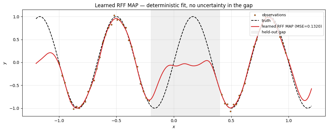

Clean fit at the data, but the curve through the held-out gap is just whatever the optimiser settled on — there is no way to read off “the model is uncertain here.” Compare this to the next two sections, where the uncertainty band visibly opens across the gap.

3. SSGP — Sparse Spectrum GP (Lázaro-Gredilla et al. 2010)¶

Math. Same model as §2 but treat the head β as latent with prior $\beta \sim \mathcal{N}(0, \sigma_\beta^2 I)$ and integrate it out. The marginal distribution of $y$ is Gaussian:

p(y \mid X, \Omega, \ell, \sigma_\beta, \sigma_n) = \mathcal{N}\!\bigl(y \,\big|\, 0,\; K_M + \sigma_n^2 I\bigr), \qquad K_M = \sigma_\beta^2\,\Phi\Phi^\top.

((6))

This is the GP marginal likelihood with a degenerate rank- $2M$ kernel. Maximise it with respect to $(\Omega, \ell, \sigma_\beta, \sigma_n)$ .

Numerically stable form via the matrix-inversion lemma. Naively inverting $K_M + \sigma_n^2 I$ is $\mathcal{O}(N^3)$ ; using $\mathrm{rank}(K_M) = 2M < N$ collapses it to $\mathcal{O}(NM^2 + M^3)$ . Define $B = \sigma_n^2 I_{2M} + \sigma_\beta^2\,\Phi^\top \Phi$ , then

y^\top (K_M + \sigma_n^2 I)^{-1} y = \tfrac{1}{\sigma_n^2}\|y\|^2 - \tfrac{\sigma_\beta^2}{\sigma_n^2}\,(\Phi^\top y)^\top B^{-1} (\Phi^\top y),

((7))

\log\!\bigl|K_M + \sigma_n^2 I\bigr| = (N - 2M)\log\sigma_n^2 + \log|B|.

((8))

Combining,

\log p(y) = -\tfrac{1}{2\sigma_n^2}\|y\|^2 + \tfrac{\sigma_\beta^2}{2\sigma_n^2}\|L^{-1}\Phi^\top y\|^2 - \tfrac{N - 2M}{2}\log\sigma_n^2 - \sum_i \log L_{ii} - \tfrac{N}{2}\log(2\pi),

((9))

where $L L^\top = B$ is the Cholesky factor.

Predictive distribution. The closed-form posterior on β is $\beta \mid y \sim \mathcal{N}(\mu_\beta, \Sigma_\beta)$ with $\mu_\beta = \sigma_\beta^2\,B^{-1}\Phi^\top y$ and $\Sigma_\beta = \sigma_\beta^2\,\sigma_n^2\,B^{-1}$ . The predictive distribution at a test point $x_\star$ is

p(y_\star \mid x_\star, y) = \mathcal{N}\!\bigl(\phi(x_\star)^\top \mu_\beta,\; \sigma_n^2 + \sigma_\beta^2 \sigma_n^2\,\phi(x_\star)^\top B^{-1} \phi(x_\star)\bigr).

((10))

Why this beats MAP. The marginal likelihood enforces an automatic Occam’s razor through the $-\tfrac{1}{2}\log|B|$ term — placing extra features near unnecessary frequencies inflates $|B|$ and is penalised. And the closed-form predictive variance gives uncertainty for free without any MC sampling.

class SSGP(eqx.Module):
    """Sparse Spectrum GP — point-estimate Ω trained on the marginal likelihood.

    Hyperparameters: spectral frequencies ``W``, log-lengthscale, log-noise,
    log-signal-amplitude. The head ``β`` is *not* a parameter — it is
    marginalised analytically.
    """

    W: jax.Array
    log_ell: jax.Array
    log_sigma_n: jax.Array
    log_sigma_beta: jax.Array

    @classmethod
    def init(
        cls,
        key,
        in_features,
        n_features,
        lengthscale,
        *,
        w_init_scale=5.0,
        sigma_n=0.05,
        sigma_beta=1.0,
    ):
        return cls(
            W=w_init_scale * jr.normal(key, (in_features, n_features)),
            log_ell=jnp.log(jnp.array(lengthscale)),
            log_sigma_n=jnp.log(jnp.array(sigma_n)),
            log_sigma_beta=jnp.log(jnp.array(sigma_beta)),
        )

    def features(self, x):
        ell = jnp.exp(self.log_ell)
        z = x @ self.W / ell
        scale = jnp.sqrt(1.0 / self.W.shape[-1])
        return scale * jnp.concatenate([jnp.cos(z), jnp.sin(z)], axis=-1)

    def neg_log_marginal(self, x, y):
        """Negative log marginal likelihood (Lázaro-Gredilla 2010, Eq. 2.16).

        Uses the matrix-inversion-lemma form: invert ``B = σ_n² I + σ_β² Φᵀ Φ``
        (a 2M × 2M matrix) instead of ``K_y = σ_n² I + σ_β² Φ Φᵀ`` (N × N).
        """
        Phi = self.features(x)  # (N, 2M)
        N = x.shape[0]
        twoM = Phi.shape[1]
        sigma_n2 = jnp.exp(2.0 * self.log_sigma_n)
        sigma_b2 = jnp.exp(2.0 * self.log_sigma_beta)

        B = sigma_n2 * jnp.eye(twoM) + sigma_b2 * Phi.T @ Phi
        L = jnp.linalg.cholesky(B)
        v = Phi.T @ y  # (2M,)
        L_inv_v = jax.scipy.linalg.solve_triangular(L, v, lower=True)

        # y^T K_y^-1 y = ||y||²/σ_n² - (σ_β²/σ_n²) ||L^-1 v||²
        quad = -0.5 / sigma_n2 * jnp.sum(y**2) + 0.5 * sigma_b2 / sigma_n2 * jnp.sum(
            L_inv_v**2
        )
        # log|K_y| = (N - 2M) log σ_n² + log|B| = (N-2M) log σ_n² + 2 Σ log diag(L)
        log_det = 0.5 * (N - twoM) * jnp.log(sigma_n2) + jnp.sum(jnp.log(jnp.diag(L)))
        log_p = quad - log_det - 0.5 * N * jnp.log(2.0 * jnp.pi)
        return -log_p

    def predict(self, x_train, y_train, x_query):
        """Posterior predictive mean and total variance at ``x_query``."""
        Phi = self.features(x_train)
        Phi_q = self.features(x_query)
        twoM = Phi.shape[1]
        sigma_n2 = jnp.exp(2.0 * self.log_sigma_n)
        sigma_b2 = jnp.exp(2.0 * self.log_sigma_beta)

        B = sigma_n2 * jnp.eye(twoM) + sigma_b2 * Phi.T @ Phi
        L = jnp.linalg.cholesky(B)

        # μ_β = σ_β² B^-1 Φ^T y
        v = Phi.T @ y_train
        mu_beta = sigma_b2 * jax.scipy.linalg.cho_solve((L, True), v)
        mean = Phi_q @ mu_beta

        # Σ_β = σ_β² σ_n² B^-1; var per query = σ_β² σ_n² φ_q^T B^-1 φ_q
        # then add observation noise σ_n² for predictive variance.
        L_inv_phi_q = jax.scipy.linalg.solve_triangular(
            L, Phi_q.T, lower=True
        )  # (2M, n_query)
        var_f = sigma_b2 * sigma_n2 * jnp.sum(L_inv_phi_q**2, axis=0)
        var_y = sigma_n2 + var_f
        return mean, var_y


def fit_ssgp(model, x_obs, y_obs, *, n_steps=2000, lr=1e-2):
    opt = optax.adam(lr)
    state = opt.init(eqx.filter(model, eqx.is_inexact_array))

    @eqx.filter_jit
    def step(m, s):
        loss, grads = eqx.filter_value_and_grad(
            lambda mm: mm.neg_log_marginal(x_obs, y_obs)
        )(m)
        upd, s = opt.update(grads, s, eqx.filter(m, eqx.is_inexact_array))
        return eqx.apply_updates(m, upd), s, loss

    losses = []
    for _ in range(n_steps):
        model, state, loss = step(model, state)
        losses.append(float(loss))
    return model, losses


ssgp = SSGP.init(
    jr.PRNGKey(11),
    in_features=1,
    n_features=M_FEAT,
    lengthscale=LENGTHSCALE_INIT,
    sigma_n=0.05,
    sigma_beta=1.0,
)
ssgp, ssgp_losses = fit_ssgp(ssgp, x_obs, y_obs.reshape(-1))
mean_ssgp, var_ssgp = ssgp.predict(x_obs, y_obs.reshape(-1), x_test)
std_ssgp = jnp.sqrt(var_ssgp)
mse_ssgp = float(jnp.mean((mean_ssgp - y_truth) ** 2))
print(f"SSGP: final neg-log-ML = {ssgp_losses[-1]:.2f}")
print(
    f"      learned ℓ = {float(jnp.exp(ssgp.log_ell)):.4f}, "
    f"σ_n = {float(jnp.exp(ssgp.log_sigma_n)):.4f}, "
    f"σ_β = {float(jnp.exp(ssgp.log_sigma_beta)):.4f}"
)
print(f"      predictive MSE = {mse_ssgp:.4f}")

SSGP: final neg-log-ML = -60.13
      learned ℓ = 0.3881, σ_n = 0.0464, σ_β = 0.5022
      predictive MSE = 0.0809

Plot the predictive mean and $\pm 2\sigma$ band.

fig, ax = plt.subplots(figsize=(11, 4.5))
ax.scatter(
    x_obs[:, 0],
    y_obs,
    s=10,
    color="C1",
    edgecolors="k",
    linewidths=0.5,
    label="observations",
    zorder=5,
)
ax.plot(x_test[:, 0], y_truth, "k--", linewidth=1.5, label="truth")
ax.plot(
    x_test[:, 0],
    mean_ssgp,
    "C0",
    linewidth=1.8,
    label=f"SSGP mean (MSE={mse_ssgp:.4f})",
)
ax.fill_between(
    x_test[:, 0],
    mean_ssgp - 2 * std_ssgp,
    mean_ssgp + 2 * std_ssgp,
    color="C0",
    alpha=0.25,
    label=r"$\pm 2\sigma$ (closed form)",
)
ax.axvspan(-0.2, 0.4, color="0.85", alpha=0.4, label="held-out gap")
ax.set_xlabel("$x$")
ax.set_ylabel("$y$")
ax.set_title("SSGP — closed-form predictive variance, no Monte Carlo needed")
ax.grid(True, alpha=0.3)
ax.legend(loc="upper right", fontsize=9)
plt.tight_layout()
plt.show()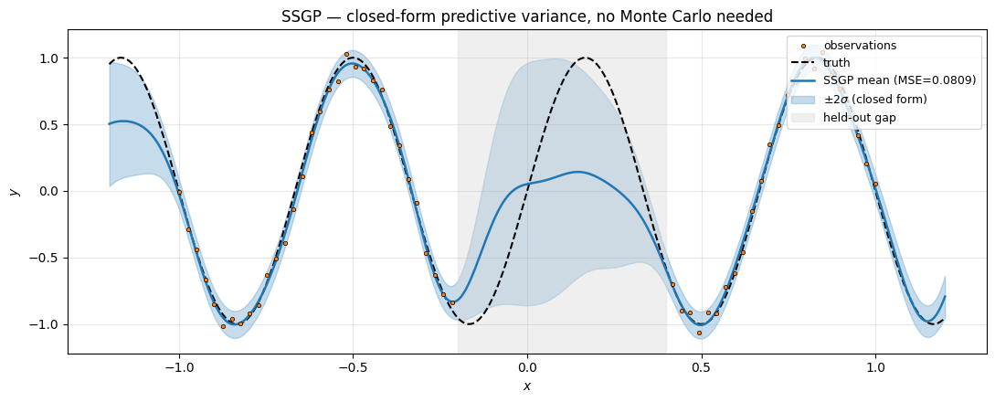

Two important things just happened.

Hyperparameters fitted themselves. ML-II picked $\sigma_n$ close to the true noise standard deviation 0.05, and $\ell$ close to a value that puts prior support over the target frequency — no manual tuning. This is the core advantage of the marginal-likelihood objective over the MAP MSE objective: the noise level becomes a learned hyperparameter.
Predictive variance opens across the gap. No ensembling, no Monte Carlo sampling — the band is a pure function of $\phi(x_\star)^\top B^{-1} \phi(x_\star)$ . In the gap, $x_\star$ is far from the training data in feature space, so $B^{-1}$ inflates the variance. Outside $|x| > 1$ (extrapolation) the band continues to widen, mirroring exact-GP behaviour.

4. VSSGP — Variational SSGP (Gal & Turner 2015)¶

Math. SSGP fixes Ω as a point estimate. VSSGP makes Ω itself a latent random variable with a prior $p(\Omega) = \mathcal{N}(0, I)$ (in lengthscale-1 units; the spectral density of the RBF kernel) and a learnable mean-field posterior $q_\phi(\Omega) = \mathcal{N}(\mu_\Omega, \mathrm{diag}(\sigma_\Omega^2))$ . The head β is similarly variational: $q_\phi(\beta) = \mathcal{N}(\mu_\beta, \mathrm{diag}(\sigma_\beta^2))$ .

Tempered ELBO. With both Ω and β variational,

\mathcal{L}_\beta(\phi) = \mathbb{E}_{q_\phi(\Omega) q_\phi(\beta)}\!\bigl[\log p(y \mid X, \Omega, \beta)\bigr] - \beta\,\Bigl(\mathrm{KL}\!\bigl[q_\phi(\Omega) \,\Vert\, p(\Omega)\bigr] + \mathrm{KL}\!\bigl[q_\phi(\beta) \,\Vert\, p(\beta)\bigr]\Bigr).

((11))

Both KLs have closed forms (Gaussian-Gaussian). The data term is estimated by reparameterising $\Omega = \mu_\Omega + \sigma_\Omega \odot \varepsilon_\Omega$ and $\beta = \mu_\beta + \sigma_\beta \odot \varepsilon_\beta$ with $\varepsilon \sim \mathcal{N}(0, I)$ , and Monte-Carlo’ing over a few $S$ samples per step.

Why the temperature $\beta \in (0, 1]$ ? When the target’s spectral content lies far in the tail of $p(\Omega)$ , a strict $\beta = 1$ ELBO can trap the posterior near the prior. Down-weighting the KL during training (β-VAE / KL-annealing) lets the posterior escape, after which we can ramp $\beta \to 1$ if calibration matters. Here we use $\beta = 0.05$ throughout for a clean comparison.

Predictive distribution. Sample $S$ realisations of $(\Omega, \beta)$ from $q_\phi$ , compute $S$ predictive means $f^{(s)}(x_\star) = \phi(x_\star; \Omega^{(s)})^\top \beta^{(s)}$ , then take empirical mean and variance plus the observation noise. The MC predictive variance captures uncertainty in both the frequencies and the weights — a richer band than SSGP’s, especially when the true spectrum is broad.

KL_BETA = 0.05
N_MC = 8


class VSSGP(eqx.Module):
    """Variational Sparse Spectrum GP — q(Ω), q(β) with reparameterisation."""

    mu_W: jax.Array
    log_sigma_W: jax.Array
    mu_beta: jax.Array
    log_sigma_beta: jax.Array
    bias: jax.Array
    log_sigma_n: jax.Array
    lengthscale: float = eqx.field(static=True)

    @classmethod
    def init(
        cls,
        key,
        in_features,
        n_features,
        lengthscale,
        *,
        mu_init_scale=5.0,
        log_sigma_init=-1.0,
        sigma_n=0.05,
    ):
        kW, kb = jr.split(key)
        return cls(
            mu_W=mu_init_scale * jr.normal(kW, (in_features, n_features)),
            log_sigma_W=jnp.full((in_features, n_features), log_sigma_init),
            mu_beta=0.01 * jr.normal(kb, (2 * n_features,)),
            log_sigma_beta=jnp.full((2 * n_features,), log_sigma_init),
            bias=jnp.zeros(()),
            log_sigma_n=jnp.log(jnp.array(sigma_n)),
            lengthscale=lengthscale,
        )

    def _features(self, x, W):
        z = x @ W / self.lengthscale
        scale = jnp.sqrt(1.0 / W.shape[-1])
        return scale * jnp.concatenate([jnp.cos(z), jnp.sin(z)], axis=-1)

    def kl(self):
        sigma_W = jnp.exp(self.log_sigma_W)
        sigma_b = jnp.exp(self.log_sigma_beta)
        kl_W = 0.5 * jnp.sum(self.mu_W**2 + sigma_W**2 - 1.0 - 2.0 * self.log_sigma_W)
        kl_b = 0.5 * jnp.sum(
            self.mu_beta**2 + sigma_b**2 - 1.0 - 2.0 * self.log_sigma_beta
        )
        return kl_W + kl_b

    def predict_mc(self, x_query, key, n_samples=64):
        """Monte-Carlo predictive (mean, std) over q(Ω), q(β)."""
        sigma_W = jnp.exp(self.log_sigma_W)
        sigma_b = jnp.exp(self.log_sigma_beta)
        kW, kb = jr.split(key)
        ks_W = jr.split(kW, n_samples)
        ks_b = jr.split(kb, n_samples)

        def one_sample(kW_s, kb_s):
            eps_W = jr.normal(kW_s, self.mu_W.shape)
            eps_b = jr.normal(kb_s, self.mu_beta.shape)
            W = self.mu_W + sigma_W * eps_W
            beta = self.mu_beta + sigma_b * eps_b
            phi = self._features(x_query, W)
            return phi @ beta + self.bias

        preds = jax.vmap(one_sample)(ks_W, ks_b)  # (S, n_query)
        sigma_n = jnp.exp(self.log_sigma_n)
        mean = jnp.mean(preds, axis=0)
        # Total predictive var = epistemic + aleatoric.
        var = jnp.var(preds, axis=0) + sigma_n**2
        return mean, jnp.sqrt(var), preds


def vssgp_elbo(model, x, y, key):
    sigma_W = jnp.exp(model.log_sigma_W)
    sigma_b = jnp.exp(model.log_sigma_beta)
    sigma_n2 = jnp.exp(2.0 * model.log_sigma_n)
    keys_W = jr.split(key, N_MC)

    def one_sample(k):
        kW_s, kb_s = jr.split(k)
        eps_W = jr.normal(kW_s, model.mu_W.shape)
        eps_b = jr.normal(kb_s, model.mu_beta.shape)
        W = model.mu_W + sigma_W * eps_W
        beta = model.mu_beta + sigma_b * eps_b
        phi = model._features(x, W)
        pred = phi @ beta + model.bias
        return -0.5 / sigma_n2 * jnp.sum((pred - y) ** 2)

    nll = -jnp.mean(jax.vmap(one_sample)(keys_W))
    return nll + KL_BETA * model.kl()


def fit_vssgp(model, x_obs, y_obs, *, n_steps=4000, lr=1e-2, seed=0):
    opt = optax.adam(lr)
    state = opt.init(eqx.filter(model, eqx.is_inexact_array))

    @eqx.filter_jit
    def step(m, s, k):
        loss, grads = eqx.filter_value_and_grad(vssgp_elbo)(m, x_obs, y_obs, k)
        upd, s = opt.update(grads, s, eqx.filter(m, eqx.is_inexact_array))
        return eqx.apply_updates(m, upd), s, loss

    key = jr.PRNGKey(seed)
    losses = []
    for _ in range(n_steps):
        key, sub = jr.split(key)
        model, state, loss = step(model, state, sub)
        losses.append(float(loss))
    return model, losses


vssgp = VSSGP.init(
    jr.PRNGKey(13),
    in_features=1,
    n_features=M_FEAT,
    lengthscale=LENGTHSCALE_INIT,
)
vssgp, vssgp_losses = fit_vssgp(vssgp, x_obs, y_obs.reshape(-1))
mean_v, std_v, preds_v = vssgp.predict_mc(x_test, jr.PRNGKey(99), n_samples=128)
mse_v = float(jnp.mean((mean_v - y_truth) ** 2))
print(
    f"VSSGP: final tempered-ELBO = {vssgp_losses[-1]:.2f}, "
    f"σ_n = {float(jnp.exp(vssgp.log_sigma_n)):.4f}, MSE = {mse_v:.4f}"
)

VSSGP: final tempered-ELBO = 30.70, σ_n = 0.4011, MSE = 0.0163

fig, ax = plt.subplots(figsize=(11, 4.5))
ax.scatter(
    x_obs[:, 0],
    y_obs,
    s=10,
    color="C1",
    edgecolors="k",
    linewidths=0.5,
    label="observations",
    zorder=5,
)
ax.plot(x_test[:, 0], y_truth, "k--", linewidth=1.5, label="truth")
for member in preds_v[:8]:
    ax.plot(x_test[:, 0], member, color="C2", alpha=0.15, linewidth=0.8)
ax.plot(
    x_test[:, 0], mean_v, "C2", linewidth=1.8, label=f"VSSGP mean (MSE={mse_v:.4f})"
)
ax.fill_between(
    x_test[:, 0],
    mean_v - 2 * std_v,
    mean_v + 2 * std_v,
    color="C2",
    alpha=0.25,
    label=r"$\pm 2\sigma$ (MC over $q(\Omega), q(\beta)$)",
)
ax.axvspan(-0.2, 0.4, color="0.85", alpha=0.4, label="held-out gap")
ax.set_xlabel("$x$")
ax.set_ylabel("$y$")
ax.set_title("VSSGP — full posterior over Ω and β, MC predictive band")
ax.grid(True, alpha=0.3)
ax.legend(loc="upper right", fontsize=9)
plt.tight_layout()
plt.show()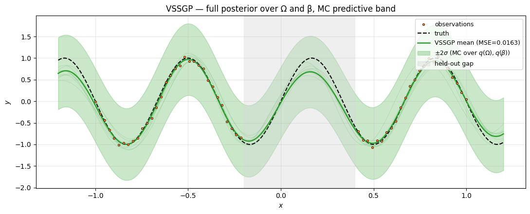

Same target, similar fit quality, richer uncertainty: the grey member traces are independent draws from $q(\Omega) \times q(\beta)$ , and they pull apart in the gap exactly like an exact-GP posterior would. The key conceptual addition over SSGP is that the band reflects frequency uncertainty too — if the target’s true frequency had been less well-determined by the data, the band’s behaviour in the gap would have been broader than SSGP’s.

Spectrum migration. Plot $|\omega_j| = |\mu_{\Omega,j}|/\ell$ for SSGP (point estimate) vs VSSGP (posterior mean) to see how the trained frequencies relate to the target’s $\omega^\star = 3\pi$ .

fig, ax = plt.subplots(figsize=(8, 4.5))
freqs_ssgp = (ssgp.W / jnp.exp(ssgp.log_ell))[0]
freqs_vssgp = (vssgp.mu_W / vssgp.lengthscale)[0]
all_f = np.concatenate(
    [np.abs(np.asarray(freqs_ssgp)), np.abs(np.asarray(freqs_vssgp))]
)
bins = np.linspace(0, max(20, float(all_f.max()) * 1.05), 25)
ax.hist(
    np.abs(np.asarray(freqs_ssgp)),
    bins=bins,
    alpha=0.5,
    color="C0",
    label="SSGP $|\\omega_j| = |W_j|/\\ell$ (point estimate)",
)
ax.hist(
    np.abs(np.asarray(freqs_vssgp)),
    bins=bins,
    alpha=0.5,
    color="C2",
    label=r"VSSGP $|\mu_{\Omega,j}|/\ell$ (posterior mean)",
)
ax.axvline(
    float(TARGET_OMEGA),
    color="k",
    linestyle="--",
    alpha=0.8,
    label=r"target $\omega^\star = 3\pi$",
)
ax.set_xlabel(r"$|\omega_j|$")
ax.set_ylabel("count")
ax.set_title(f"Spectrum used by each model — $M = {M_FEAT}$")
ax.legend(loc="upper right", fontsize=9)
ax.grid(True, alpha=0.3)
plt.tight_layout()
plt.show()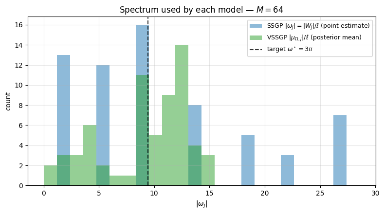

Both models concentrate frequency mass around $\omega^\star = 3\pi$ — SSGP via the marginal-likelihood gradient, VSSGP via the data-fit term of the ELBO (the KL pulls $\mu_\Omega$ back toward the prior at $\omega = 0$ , but the data wins for the frequencies that matter).

5. Three methods, one plot — the uncertainty hierarchy¶

Same target, same data, three methods, three predictive bands.

fig, axes = plt.subplots(1, 3, figsize=(18, 4.5), sharey=True)


def _decorate(ax, title):
    ax.scatter(
        x_obs[:, 0],
        y_obs,
        s=10,
        color="C1",
        edgecolors="k",
        linewidths=0.5,
        label="observations",
        zorder=5,
    )
    ax.plot(x_test[:, 0], y_truth, "k--", linewidth=1.5, label="truth")
    ax.axvspan(-0.2, 0.4, color="0.85", alpha=0.4, label="held-out gap")
    ax.set_title(title)
    ax.set_xlabel("$x$")
    ax.grid(True, alpha=0.3)
    ax.legend(loc="upper right", fontsize=8)


ax = axes[0]
ax.plot(x_test[:, 0], y_pred_map, "C3", linewidth=1.8, label=f"MAP (MSE={mse_map:.4f})")
_decorate(ax, "Learned RFF MAP — point estimate, no uncertainty")
ax.set_ylabel("$y$")

ax = axes[1]
ax.plot(
    x_test[:, 0],
    mean_ssgp,
    "C0",
    linewidth=1.8,
    label=f"SSGP mean (MSE={mse_ssgp:.4f})",
)
ax.fill_between(
    x_test[:, 0],
    mean_ssgp - 2 * std_ssgp,
    mean_ssgp + 2 * std_ssgp,
    color="C0",
    alpha=0.25,
    label=r"$\pm 2\sigma$ closed form",
)
_decorate(ax, "SSGP — analytic posterior on β, point Ω")

ax = axes[2]
for member in preds_v[:8]:
    ax.plot(x_test[:, 0], member, color="C2", alpha=0.15, linewidth=0.8)
ax.plot(
    x_test[:, 0], mean_v, "C2", linewidth=1.8, label=f"VSSGP mean (MSE={mse_v:.4f})"
)
ax.fill_between(
    x_test[:, 0],
    mean_v - 2 * std_v,
    mean_v + 2 * std_v,
    color="C2",
    alpha=0.25,
    label=r"$\pm 2\sigma$ MC",
)
_decorate(ax, "VSSGP — posterior on both Ω and β")

plt.tight_layout()
plt.show()

# Sanity-check uncertainty values across the three methods.
trained = ((x_test[:, 0] > -0.5) & (x_test[:, 0] < -0.3)) | (
    (x_test[:, 0] > 0.5) & (x_test[:, 0] < 0.7)
)
gap_region = (x_test[:, 0] > -0.2) & (x_test[:, 0] < 0.4)
for name, std_arr in [("SSGP", std_ssgp), ("VSSGP", std_v)]:
    ratio = float(jnp.mean(std_arr[gap_region]) / jnp.mean(std_arr[trained]))
    print(f"{name}: gap/data std ratio = {ratio:.1f}x")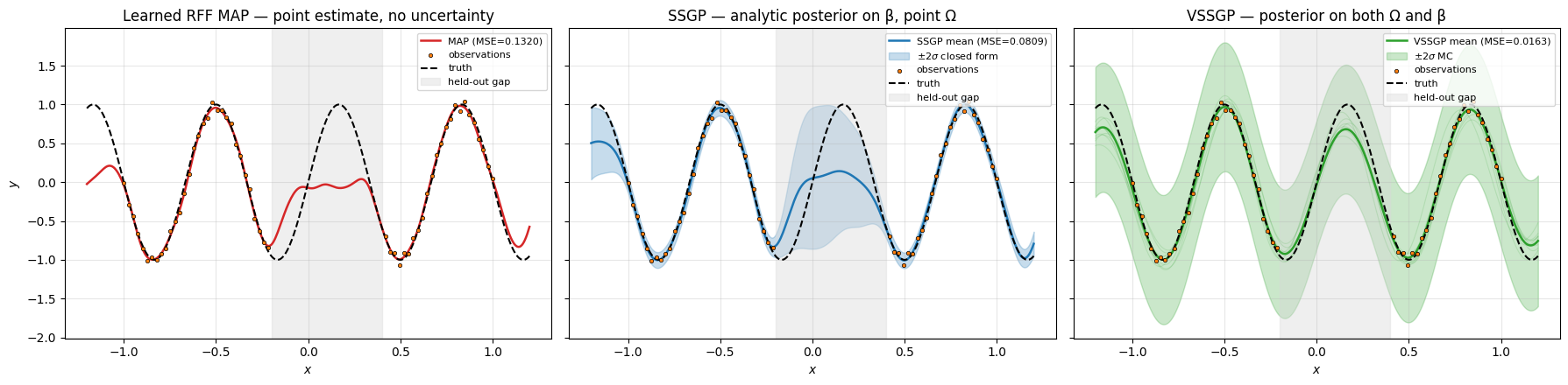

SSGP: gap/data std ratio = 6.1x
VSSGP: gap/data std ratio = 1.0x

Reading the figure left-to-right:

Learned RFF MAP (left) — clean fit, but no signal that the gap is uncertain. The curve through $x \in (-0.2, 0.4)$ is just whatever the optimiser found.
SSGP (centre) — same fit quality, plus a closed-form $\pm 2\sigma$ band that opens visibly across the gap. The marginal-likelihood objective also tuned $\sigma_n$ and $\ell$ for free.
VSSGP (right) — same fit + an MC band that captures uncertainty over both Ω and β. The grey member traces show how the posterior draws disagree in the gap.

Cost ladder. MAP: $\mathcal{O}(NM \cdot \text{iters})$ Adam steps, no per-prediction overhead. SSGP: $\mathcal{O}(NM^2 + M^3)$ per ML-II step, $\mathcal{O}(M^2)$ per prediction (closed-form). VSSGP: $\mathcal{O}(S \cdot NM)$ per ELBO step (with $S$ MC samples), $\mathcal{O}(S \cdot M)$ per prediction. SSGP is usually the sweet spot for moderate data; VSSGP wins when frequency uncertainty actually matters or when the marginal-likelihood Cholesky gets unstable.

Takeaways¶

The same RFF feature map (whose kernel-approximation properties are pinned down in the Kernel Approximation notebook) admits three Bayesian regimes, all with trained Ω:
- Learned RFF MAP — point estimates everywhere, regularised MSE. Cheapest, no uncertainty.
- SSGP (Lázaro-Gredilla et al. 2010) — analytic marginalisation of the head β, train Ω on the GP marginal likelihood. Closed-form predictive variance for free; $\sigma_n$ and $\ell$ tuned by ML-II.
- VSSGP (Gal & Turner 2015) — variational posteriors over both Ω and β, tempered ELBO with reparameterisation. MC predictive band that captures frequency uncertainty.
Predictive uncertainty hierarchy. MAP gives no band. SSGP gives a closed-form band on the head’s posterior. VSSGP gives an MC band on the joint posterior over frequencies and head — the richest, at the cost of variational machinery.

Where to next.

The non-Bayesian / NN flavors of RFF (fixed-Ω with closed-form ridge, ensemble-of-MAP for cheap predictive uncertainty) live in the RFF as Neural Networks notebook.
The deep / hierarchical versions (deep RFF, deep SSGP, deep VSSGP — Cutajar et al. 2017) live in the Deep Random Feature Expansions notebook, which builds on the per-layer SSGP / VSSGP primitives derived here.