L96 benchmark — analysis-then-forecast across 10 Lyapunov times
Every method assimilates obs on the 0.5-time-unit window then is free-forecast for 4.5 more time units (10 L96 Lyapunov times total). The Hovmöller plots and the RMSE(t) trace below are directly comparable to PyDA’s L96 EnKF demo.
from __future__ import annotations

import time

import equinox as eqx
import jax
import jax.numpy as jnp
import lineax as lx
import matplotlib.pyplot as plt
import optax
import vardax as vdx

from assimilation import (
    Lorenz96Forward,
    assemble_full_trajectory,
    assim_batch,
    compare,
    generate_l96_problem,
    run_method,
)
1. Shared problem
prob = generate_l96_problem(key=jax.random.PRNGKey(0))
batch = assim_batch(prob)
fwd = Lorenz96Forward(K=prob.K, F=prob.F, dt=prob.dt)
H_full = lx.IdentityLinearOperator(
    jax.ShapeDtypeStruct(prob.prior_mean.shape, jnp.float32)
)
H_state = lx.IdentityLinearOperator(jax.ShapeDtypeStruct((prob.K,), jnp.float32))
t_axis = jnp.arange(prob.T_total_plus_1) * prob.dt
print(f"K={prob.K}, T_assim={prob.T_assim}, T_total={prob.T_total}")
print(f"obs in assim window: {int(prob.mask.sum())} scalars")
K=40, T_assim=50, T_total=250
obs in assim window: 110 scalars
2. Classical methods
oi = vdx.OptimalInterpolation(
    obs_op=vdx.LinearObs(H_mat=H_full),
    prior_mean=prob.prior_mean, prior_cov_op=prob.B_op, obs_cov_op=prob.R_op,
)
three = vdx.ThreeDVar(
    obs_op=vdx.LinearObs(H_mat=H_full),
    prior_mean=prob.prior_mean, prior_cov_op=prob.B_op, obs_cov_op=prob.R_op,
    max_steps=1000,
)
strong = vdx.StrongFourDVar(
    forward=fwd, obs_op=vdx.LinearObs(H_mat=H_state),
    prior_mean=prob.prior_mean_state, prior_cov_op=prob.B_op_state,
    obs_cov_op=prob.R_op_state, max_steps=2000,
)
inc = vdx.IncrementalFourDVar(
    forward=fwd, obs_op=vdx.LinearObs(H_mat=H_state),
    prior_mean=prob.prior_mean_state, prior_cov_op=prob.B_op_state,
    obs_cov_op=prob.R_op_state,
    config=vdx.IncrementalConfig(n_outer=4, n_inner=200,
                                 cg_atol=1e-3, cg_rtol=1e-3),
)

results = [
    run_method("oi",
               lambda: assemble_full_trajectory(oi(batch)[0], prob, fwd), prob),
    run_method("3dvar",
               lambda: assemble_full_trajectory(three(batch)[0], prob, fwd), prob),
    run_method("strong_4dvar",
               lambda: assemble_full_trajectory(strong(batch)[0], prob, fwd), prob),
    run_method("incremental_4dvar",
               lambda: assemble_full_trajectory(inc(batch)[0], prob, fwd), prob),
]
for r in results:
    print(f"{r.name:20s} assim={r.rmse_assim:7.3f}  "
          f"forecast={r.rmse_forecast:7.3f}  total={r.rmse_total:7.3f}")
oi assim= 3.925 forecast= 4.212 total= 4.156
3dvar assim= 3.925 forecast= 4.212 total= 4.156
strong_4dvar assim= 3.744 forecast= 4.142 total= 4.064
incremental_4dvar assim= 4.629 forecast= 5.121 total= 5.025
3. Learned methods
def make_pair(k):
    p = generate_l96_problem(key=k)
    return p.obs, p.mask, p.truth[: prob.T_assim_plus_1]


# FourDVarNet
key = jax.random.PRNGKey(0)
fvn = vdx.FourDVarNet1D(
    state_dim=prob.K, n_time=prob.T_assim_plus_1,
    latent_dim=32, hidden_dim=64, n_solver_steps=8, key=key,
)
fvn_keys = jax.random.split(jax.random.PRNGKey(1), 64)
obs_train, mask_train, truth_train = jax.vmap(make_pair)(fvn_keys)
fvn_batch = vdx.Batch1D(input=obs_train, mask=mask_train, target=truth_train)
fvn_opt = optax.adam(5e-3)
fvn_opt_state = fvn_opt.init(eqx.filter(fvn, eqx.is_array))
t0 = time.perf_counter()
for _ in range(500):
    fvn, fvn_opt_state, _ = vdx.train_step(fvn, fvn_batch, fvn_opt, fvn_opt_state)
fvn_train_time = time.perf_counter() - t0

results.append(run_method(
    "fourdvarnet",
    lambda: assemble_full_trajectory(fvn(batch)[0], prob, fwd),
    prob, train_time_s=fvn_train_time,
))
print(f"FourDVarNet train: {fvn_train_time:.1f}s, "
      f"rmse_forecast={results[-1].rmse_forecast:.3f}")

# Amortized
k_enc, k_head = jax.random.split(jax.random.PRNGKey(0))
amort = vdx.AmortizedPosterior(
    encoder=vdx.MLPObsEncoder(
        input_size=prob.T_assim_plus_1 * prob.K, context_dim=96,
        hidden_dim=256, depth=2, key=k_enc,
    ),
    head=vdx.RegressionHead(
        context_dim=96, state_shape=(prob.T_assim_plus_1, prob.K),
        hidden_dim=256, depth=2, key=k_head,
    ),
    config=vdx.AmortizedConfig(head_type="regression"),
)
am_keys = jax.random.split(jax.random.PRNGKey(2), 128)
obs_train, mask_train, truth_train = jax.vmap(make_pair)(am_keys)
am_batch = vdx.Batch1D(input=obs_train, mask=mask_train, target=truth_train)
am_opt = optax.adam(3e-3)
am_opt_state = am_opt.init(eqx.filter(amort, eqx.is_array))
t0 = time.perf_counter()
for _ in range(500):
    amort, am_opt_state, _ = vdx.amortized_train_step(
        amort, am_batch, am_opt, am_opt_state,
    )
am_train_time = time.perf_counter() - t0

results.append(run_method(
    "amortized",
    lambda: assemble_full_trajectory(amort(batch)[0], prob, fwd),
    prob, train_time_s=am_train_time,
))
print(f"Amortized train: {am_train_time:.1f}s, "
      f"rmse_forecast={results[-1].rmse_forecast:.3f}")
FourDVarNet train: 100.3s, rmse_forecast=4.733
Amortized train: 7.8s, rmse_forecast=4.481
4. Comparison table
table = compare(*results).sort_values("rmse_forecast")
table
Loading...
5. Hovmöller — truth, then each method
Each panel is a (time × grid) Hovmöller diagram. Methods with good recovery produce panels that look identical to the truth across the full window; bad analyses give panels that diverge from truth after a Lyapunov time.
n = len(results)
fig, axs = plt.subplots(1 + n, 1, figsize=(11, 1.5 * (1 + n)), sharex=True)
vmax = float(jnp.max(jnp.abs(prob.truth)))
kwargs = {"aspect": "auto", "cmap": "RdBu_r", "origin": "lower",
          "vmin": -vmax, "vmax": vmax,
          "extent": (0.0, prob.T_total * prob.dt, 0, prob.K)}

axs[0].imshow(prob.truth.T, **kwargs)
axs[0].axvline(prob.T_assim * prob.dt, color="yellow", lw=2)
axs[0].set_ylabel("truth")
for ax, r in zip(axs[1:], results, strict=False):
    ax.imshow(r.mean.T, **kwargs)
    ax.axvline(prob.T_assim * prob.dt, color="yellow", lw=2)
    ax.set_ylabel(f"{r.name}\nfcast={r.rmse_forecast:.2f}")
axs[-1].set_xlabel("time")
fig.suptitle("L96 — truth + 6 method Hovmöllers (yellow line = assim/forecast boundary)")
fig.tight_layout()
plt.show()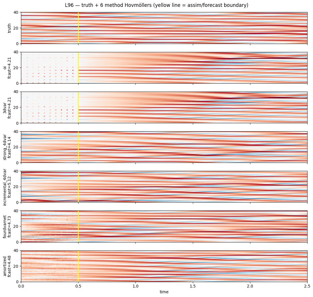
6. RMSE(t) — the dynamics view
colors = ["C0", "C1", "C2", "C4", "C5", "C6"]
fig, ax = plt.subplots(figsize=(11, 5))
ax.axvspan(0.0, prob.T_assim * prob.dt, color="yellow", alpha=0.2,
           label="assim window")
for r, c in zip(results, colors, strict=False):
    ax.plot(t_axis, r.rmse_trace, color=c, lw=1.5, label=r.name)
ax.set_xlabel("time")
ax.set_ylabel("instantaneous RMSE (log)")
ax.set_yscale("log")
ax.set_title("L96 — analysis-then-forecast RMSE trace, all methods")
ax.grid(True, alpha=0.3, which="both")
ax.legend(loc="best", fontsize=9, ncol=2)
fig.tight_layout()
plt.show()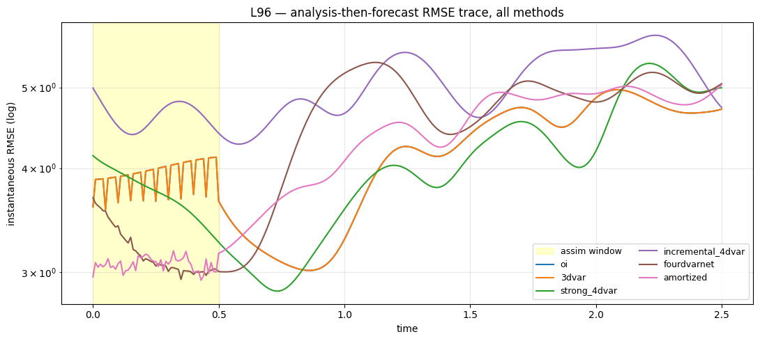
7. Headline numbers
Same story shape as L63 but with the L96 scaling: dynamics-aware methods produce launch states that hold the forecast for several Lyapunov times; OI / 3DVar’s noisy analyses produce forecasts that diverge within one Lyapunov time.