Lorenz-96 (single-level) — analysis-then-forecast setup

The higher-dimensional sibling of Lorenz-63: a ring of $K$ coupled scalar variables with periodic boundary conditions,

\frac{dx_k}{dt} = (x_{k+1} - x_{k-2})\,x_{k-1} - x_k + F.

((1))

With $K = 40$ and $F = 8$ the system is fully chaotic, with a Lyapunov time of about $1/\lambda_{\max} \approx 0.5$ time units. We use a 0.5-time-unit assim window inside a 5-time-unit total run (~10 Lyapunov times) so the free-forecast covers many e-fold times — the standard PyDA pattern, scaled to L96’s faster Lyapunov clock.

This notebook covers decisions, simulation, observation design, and sanity checks. The benchmark itself — 10_lorenz96_benchmark — runs the seven AnalysisStep methods on the resulting problem.

from __future__ import annotations

import jax
import jax.numpy as jnp
import matplotlib.pyplot as plt

from assimilation import Lorenz96Forward, generate_l96_problem

1. Decisions¶

Parameter	Value	Rationale
$K$	40	Canonical chaotic dimension.
$F$	8.0	Standard L96 chaotic forcing.
$dt$	0.01	RK4 step.
$T_\text{assim}$	50 (0.5 time units)	About one Lyapunov time; long enough for sparse obs, short enough for 4DVar’s BFGS to converge.
$T_\text{total}$	500 (5 time units)	~10 Lyapunov times of free-forecast.
$\sigma_o$	1.0	Obs noise std (~10% of typical state magnitude).
$\sigma_b$	5.0	Background-error std.

2. Simulate a long trajectory + Hovmöller¶

fwd_long = Lorenz96Forward(K=40, F=8.0, dt=0.01)
x0 = 8.0 * jnp.ones(40) + 0.01 * jax.random.normal(jax.random.PRNGKey(0), (40,))


def _scan(state, _):
    new = fwd_long.step(state, fwd_long.dt)
    return new, new


state, _ = jax.lax.scan(_scan, x0, None, length=500)  # burn-in
_, traj_long = jax.lax.scan(_scan, state, None, length=500)
print(f"long trajectory: {traj_long.shape}")

long trajectory: (500, 40)

fig, ax = plt.subplots(figsize=(10, 4))
t = jnp.arange(500) * 0.01
im = ax.imshow(
    traj_long.T, aspect="auto", cmap="RdBu_r", origin="lower",
    extent=(0, float(t[-1]), 0, 40), vmin=-12, vmax=12,
)
ax.set_xlabel("time")
ax.set_ylabel("grid index $k$")
ax.set_title("Lorenz-96 ground truth — Hovmöller diagram ($K=40$, $F=8$)")
fig.colorbar(im, ax=ax, label="$x_k$")
fig.tight_layout()
plt.show()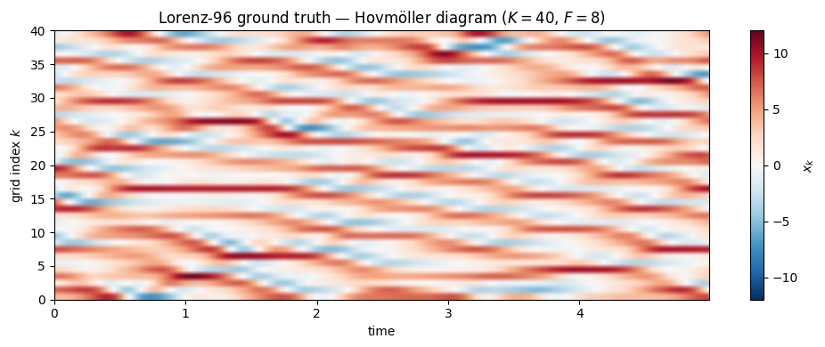

3. Observation design for forecast-mode benchmark¶

Inside the assim window: observe every 4th grid point at every 0.05 time units (every 5 model steps). 10 spatial × 11 temporal = 110 scalar obs in a 0.5-time-unit window — enough information for strong-4DVar to recover $x_0$ tightly.

Free-forecast window: no obs. Each method’s analysis is rolled forward 4.5 time units through the L96 forward.

prob = generate_l96_problem(key=jax.random.PRNGKey(0))
print(f"K={prob.K}, T_assim={prob.T_assim} (assim {prob.T_assim * prob.dt} time units)")
print(f"T_total={prob.T_total} (total {prob.T_total * prob.dt} time units)")
print(f"obs density: {int(prob.mask.sum())} / {prob.mask.size} entries in assim window")

K=40, T_assim=50 (assim 0.5 time units)
T_total=250 (total 2.5 time units)
obs density: 110 / 2040 entries in assim window

fig, axs = plt.subplots(1, 3, figsize=(13, 4), sharey=True)
extent = (0, prob.K, 0, prob.T_assim_plus_1)
for ax, field, title, cmap in zip(
    axs,
    [prob.truth[: prob.T_assim_plus_1], prob.obs, prob.mask],
    ["truth (assim window)", "observations", "binary mask"],
    ["RdBu_r", "RdBu_r", "Greys"],
    strict=False,
):
    im = ax.imshow(field, aspect="auto", cmap=cmap, origin="lower", extent=extent,
                   vmin=-12 if cmap == "RdBu_r" else None,
                   vmax=12 if cmap == "RdBu_r" else None)
    ax.set_xlabel("grid index $k$")
    ax.set_title(title)
    fig.colorbar(im, ax=ax, fraction=0.04)
axs[0].set_ylabel("time step $t$")
fig.tight_layout()
plt.show()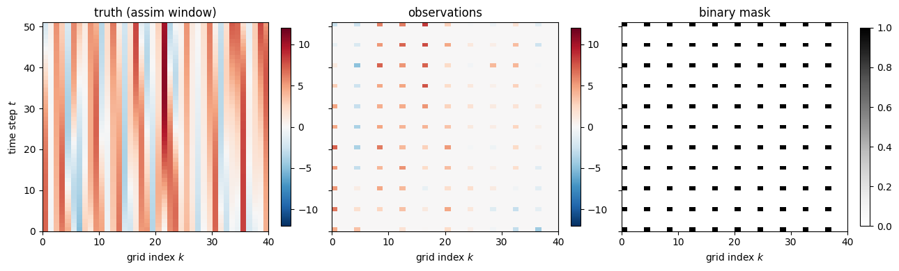

4. Forward roundtrip sanity check¶

fwd = Lorenz96Forward(K=prob.K, F=prob.F, dt=prob.dt)


def step(s, _):
    new = fwd.step(s, fwd.dt)
    return new, new


_, traj_rt = jax.lax.scan(step, prob.truth[0], None, length=prob.T_total)
truth_rt = jnp.concatenate([prob.truth[0][None, :], traj_rt], axis=0)
print(f"roundtrip max abs error: "
      f"{float(jnp.max(jnp.abs(truth_rt - prob.truth))):.2e}")

roundtrip max abs error: 0.00e+00

5. Truth Hovmöller over the full forecast window¶

10 Lyapunov times of L96 ground truth. The forecast methods aim to reconstruct this entire image from the bottom-left assim window (yellow-bordered region).

fig, ax = plt.subplots(figsize=(11, 4.5))
t_axis = jnp.arange(prob.T_total_plus_1) * prob.dt
im = ax.imshow(prob.truth.T, aspect="auto", cmap="RdBu_r", origin="lower",
               extent=(0, float(t_axis[-1]), 0, prob.K), vmin=-12, vmax=12)
ax.axvline(prob.T_assim * prob.dt, color="yellow", lw=3,
           label="assim / forecast boundary")
ax.axvspan(0, prob.T_assim * prob.dt, color="yellow", alpha=0.15)
ax.set_xlabel("time")
ax.set_ylabel("grid index $k$")
ax.set_title("L96 truth — assim window (yellow) + free-forecast horizon")
ax.legend(loc="upper right")
fig.colorbar(im, ax=ax)
fig.tight_layout()
plt.show()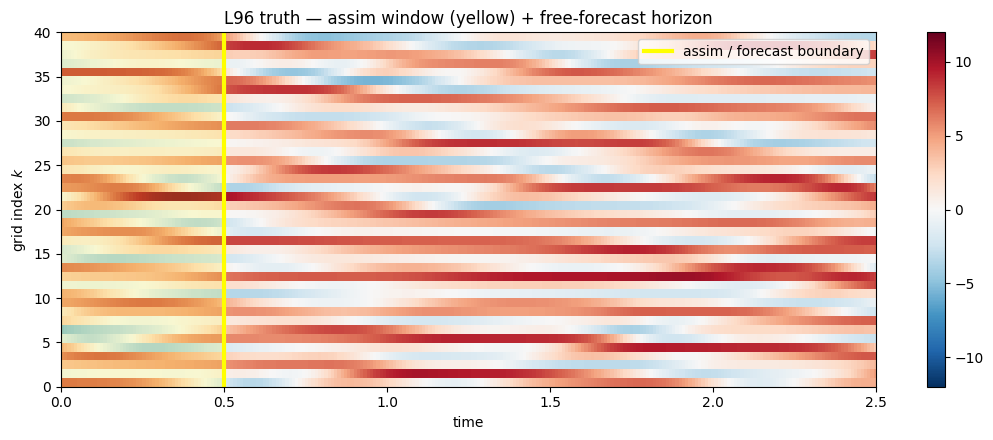

6. Next¶

Continue to 10_lorenz96_benchmark to see how each of the seven AnalysisStep methods recovers the initial state and how long the resulting forecast tracks the truth across the 10-Lyapunov-time horizon.