Markov Gaussian Processes — Matern Kernels in State-Space Form

This notebook is the first installment of pyrox’s Markov-GP track. It introduces MaternSDE — the state-space representation of the Matern-ν kernel for $\nu \in \{1/2, 3/2, 5/2\}$ — and verifies, end-to-end, that the SDE formulation and the dense kernel describe the same Gaussian process. Once a kernel is in state-space form, GP inference on a 1-D grid drops from $\mathcal{O}(N^3)$ Cholesky to $\mathcal{O}(N\,d^3)$ Kalman filtering, where $d \in \{1, 2, 3\}$ is the SDE state dimension.

Subsequent notebooks (issues #37 finish, #38) will compose SDE kernels, run Kalman / RTS smoothing, and expose MarkovGPPrior for NumPyro models. This one stays focused on the representation layer: math, identities, and visual sanity checks.

Background — from kernel to SDE¶

Any stationary GP kernel $k(\tau)$ on $\mathbb{R}$ whose spectral density is rational in $\omega^2$ admits an exact, finite-dimensional state-space representation as a linear time-invariant SDE

d\mathbf{x}(t) = F\,\mathbf{x}(t)\,dt + L\,dw(t), \qquad f(t) = H\,\mathbf{x}(t),

((1))

with white-noise driver $w(t)$ of spectral density $Q_c$ and stationary state covariance $P_\infty$ solving the continuous Lyapunov equation

F P_\infty + P_\infty F^\top + L Q_c L^\top = 0.

((2))

Discretising at non-uniform observation times $t_1 < t_2 < \dots < t_N$ with $\Delta t_k = t_{k+1} - t_k$ gives the discrete-time linear-Gaussian model

\mathbf{x}_{k+1} = A_k \mathbf{x}_k + \mathbf{q}_k, \qquad \mathbf{q}_k \sim \mathcal{N}(0, Q_k), \qquad f_k = H\,\mathbf{x}_k,

((3))

with $A_k = \exp(F\,\Delta t_k)$ and $Q_k = P_\infty - A_k P_\infty A_k^\top$ . The recovered continuous autocovariance is $k(\tau) = H \exp(F\tau) P_\infty H^\top$ for $\tau \geq 0$ , which we will verify against the dense Matern kernel below.

Matern-ν companion form¶

For Matern-ν with $\nu = p + 1/2$ and $\lambda = \sqrt{2\nu}/\ell$ , the state has dimension $d = p + 1$ and $F$ is the companion matrix of $(\lambda + s)^d$ . Concretely:

Order $p$	ν	$d$	λ	Closed-form kernel
0	1/2	1	$1/\ell$	$\sigma^2 \exp(-r/\ell)$
1	3/2	2	$\sqrt{3}/\ell$	$\sigma^2 (1 + \sqrt{3} r/\ell)\exp(-\sqrt{3} r/\ell)$
2	5/2	3	$\sqrt{5}/\ell$	$\sigma^2 (1 + \sqrt{5} r/\ell + 5 r^2/(3\ell^2))\exp(-\sqrt{5} r/\ell)$

MaternSDE ships these three orders. Composition rules (sum / product), CosineSDE, PeriodicSDE, and the Kalman-based MarkovGPPrior follow in subsequent PRs.

Setup¶

Detect Colab and install pyrox[colab] (which pulls in matplotlib and watermark) only when running there.

import subprocess
import sys


try:
    import google.colab  # noqa: F401

    IN_COLAB = True
except ImportError:
    IN_COLAB = False

if IN_COLAB:
    subprocess.run(
        [
            sys.executable,
            "-m",
            "pip",
            "install",
            "-q",
            "pyrox[colab] @ git+https://github.com/jejjohnson/pyrox@main",
        ],
        check=True,
    )

import warnings


warnings.filterwarnings("ignore", message=r".*IProgress.*")

import jax
import jax.numpy as jnp
import jax.random as jr
import jax.scipy.linalg as jsl
import matplotlib.pyplot as plt
import numpy as np

from pyrox.gp import MaternSDE
from pyrox.gp._src.kernels import matern_kernel


jax.config.update("jax_enable_x64", True)

import importlib.util


try:
    from IPython import get_ipython

    ipython = get_ipython()
except ImportError:
    ipython = None

if ipython is not None and importlib.util.find_spec("watermark") is not None:
    ipython.run_line_magic("load_ext", "watermark")
    ipython.run_line_magic("watermark", "-v -m -p jax,equinox,numpyro,pyrox,matplotlib")
else:
    print("watermark extension not installed; skipping reproducibility readout.")

Python implementation: CPython
Python version       : 3.13.5
IPython version      : 9.10.0

jax       : 0.9.2
equinox   : 0.13.6
numpyro   : 0.20.1
pyrox     : 0.0.7
matplotlib: 3.10.8

Compiler    : GCC 11.2.0
OS          : Linux
Release     : 6.8.0-1044-azure
Machine     : x86_64
Processor   : x86_64
CPU cores   : 16
Architecture: 64bit

1. Inspecting the SDE parameters¶

A MaternSDE(variance, lengthscale, order) produces a closed-form $(F, L, H, Q_c, P_\infty)$ tuple via sde_params(). We instantiate one kernel per order and print the structural matrices alongside two structural identities:

Variance recovery: $H P_\infty H^\top = \sigma^2$ .
Lyapunov closure: $F P_\infty + P_\infty F^\top + L Q_c L^\top = 0$ .

sigma2 = 1.0
ell = 0.5
sdes = {p: MaternSDE(variance=sigma2, lengthscale=ell, order=p) for p in (0, 1, 2)}

for p, sde in sdes.items():
    F, L, H, Q_c, P_inf = sde.sde_params()
    var_rec = float((H @ P_inf @ H.T).squeeze())
    lyap = F @ P_inf + P_inf @ F.T + L @ Q_c @ L.T
    print(
        f"--- Matern-{int(2 * sde.nu)}/2  (order p = {p}, state dim d = {sde.state_dim}) ---"
    )
    print(f"F =\n{np.asarray(F)}")
    print(
        f"H = {np.asarray(H).ravel()},  L^T = {np.asarray(L).ravel()},  Q_c = {float(Q_c.squeeze()):.4f}"
    )
    print(f"P_inf =\n{np.asarray(P_inf)}")
    print(f"H P_inf H^T = {var_rec:.6f}  (expected sigma^2 = {sigma2})")
    print(
        f"||F P_inf + P_inf F^T + L Q_c L^T||_inf = {float(jnp.max(jnp.abs(lyap))):.2e}"
    )
    print()

--- Matern-1/2  (order p = 0, state dim d = 1) ---
F =
[[-2.]]
H = [1.],  L^T = [1.],  Q_c = 4.0000
P_inf =
[[1.]]
H P_inf H^T = 1.000000  (expected sigma^2 = 1.0)
||F P_inf + P_inf F^T + L Q_c L^T||_inf = 0.00e+00

--- Matern-3/2  (order p = 1, state dim d = 2) ---
F =
[[  0.           1.        ]
 [-12.          -6.92820323]]
H = [1. 0.],  L^T = [0. 1.],  Q_c = 166.2769
P_inf =
[[ 1.  0.]
 [ 0. 12.]]
H P_inf H^T = 1.000000  (expected sigma^2 = 1.0)
||F P_inf + P_inf F^T + L Q_c L^T||_inf = 0.00e+00

--- Matern-5/2  (order p = 2, state dim d = 3) ---
F =
[[  0.           1.           0.        ]
 [  0.           0.           1.        ]
 [-89.4427191  -60.         -13.41640786]]
H = [1. 0. 0.],  L^T = [0. 0. 1.],  Q_c = 9540.5567
P_inf =
[[  1.           0.          -6.66666667]
 [  0.           6.66666667   0.        ]
 [ -6.66666667   0.         400.        ]]
H P_inf H^T = 1.000000  (expected sigma^2 = 1.0)
||F P_inf + P_inf F^T + L Q_c L^T||_inf = 1.68e-15

Both invariants hold to machine precision in float64. The variance-recovery identity says the SDE state encodes the GP value plus $d-1$ derivative-like coordinates; the Lyapunov identity says the stationary state covariance is consistent with the drift $F$ and the diffusion $L Q_c L^\top$ .

2. SDE autocovariance vs. dense Matern kernel¶

The continuous-time stationary autocovariance recovered from the SDE is

k_{\text{SDE}}(\tau) \;=\; H\,\exp(F \tau)\,P_\infty\,H^\top, \qquad \tau \geq 0.

((4))

This must equal the dense Matern Gram value at lag τ. We compute both on a fine grid and overlay them.

def sde_autocov(sde: MaternSDE, taus: jnp.ndarray) -> jnp.ndarray:
    F, _L, H, _Q_c, P_inf = sde.sde_params()

    def _k(tau: jnp.ndarray) -> jnp.ndarray:
        return (H @ jsl.expm(F * tau) @ P_inf @ H.T).squeeze()

    return jax.vmap(_k)(taus)


taus = jnp.linspace(0.0, 2.5, 201)
X = taus[:, None]
X0 = jnp.zeros((1, 1))

fig, axes = plt.subplots(1, 3, figsize=(13.5, 3.6), sharey=True)
for ax, (p, sde) in zip(axes, sdes.items(), strict=False):
    k_sde = sde_autocov(sde, taus)
    k_dense = matern_kernel(
        X, X0, jnp.asarray(sigma2), jnp.asarray(ell), nu=p + 0.5
    ).squeeze()
    ax.plot(taus, k_dense, label="dense Matern", lw=2.4, alpha=0.85)
    ax.plot(taus, k_sde, "--", label=r"$H \exp(F\tau) P_\infty H^\top$", lw=1.7)
    err = float(jnp.max(jnp.abs(k_sde - k_dense)))
    ax.set_title(rf"Matern-{int(2 * sde.nu)}/2 (max abs err: {err:.1e})")
    ax.set_xlabel(r"lag $\tau$")
    ax.grid(alpha=0.25)
axes[0].set_ylabel(r"$k(\tau)$")
axes[0].legend(frameon=False, loc="upper right")
fig.suptitle("SDE autocovariance recovers the dense Matern kernel")
fig.tight_layout()
plt.show()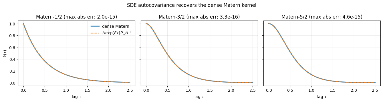

All three orders agree to numerical precision. The SDE is not an approximation of the Matern kernel — for $\nu \in \{1/2, 3/2, 5/2\}$ it is an exact reformulation.

3. Discretisation: $A_k$ and $Q_k$ as functions of $\Delta t$ ¶

Given a time step $\Delta t$ , the discrete-time transition is $A(\Delta t) = \exp(F\,\Delta t)$ and the process-noise covariance is $Q(\Delta t) = P_\infty - A(\Delta t) P_\infty A(\Delta t)^\top$ . Two endpoints are worth checking:

As $\Delta t \to 0$ , $A \to I$ and $Q \to 0$ (no time elapsed, no uncertainty added).
As $\Delta t \to \infty$ , $A P_\infty A^\top \to 0$ (the dynamics decay back to the stationary distribution) and so $Q \to P_\infty$ (the next state is independent of the previous one and has the stationary distribution).

We plot $\|A(\Delta t)\|_2$ and the trace of $Q(\Delta t)$ over a log-spaced range of step sizes.

dts = jnp.geomspace(1e-3, 5e1, 200)

fig, axes = plt.subplots(1, 2, figsize=(11, 3.6))
for p, sde in sdes.items():
    A, Q = sde.discretise(dts)
    A_norm = jnp.linalg.norm(A, ord=2, axis=(1, 2))
    Q_trace = jnp.einsum("nii->n", Q)
    _, _, _, _, P_inf = sde.sde_params()
    P_inf_trace = float(jnp.trace(P_inf))
    label = rf"$\nu = {p}+1/2$"
    axes[0].plot(dts, A_norm, label=label, lw=1.8)
    axes[1].plot(dts, Q_trace, label=label, lw=1.8)
    axes[1].axhline(
        P_inf_trace, color=axes[1].lines[-1].get_color(), ls=":", alpha=0.55
    )

for ax in axes:
    ax.set_xscale("log")
    ax.set_xlabel(r"step size $\Delta t$")
    ax.grid(alpha=0.25)
axes[0].set_ylabel(r"$\|A(\Delta t)\|_2$")
axes[0].set_title(r"Transition matrix decay: $A \to 0$ as $\Delta t \to \infty$")
axes[1].set_ylabel(r"$\mathrm{tr}\,Q(\Delta t)$")
axes[1].set_title(r"Process noise growth: $Q \to P_\infty$ as $\Delta t \to \infty$")
axes[1].legend(frameon=False, loc="lower right")
fig.tight_layout()
plt.show()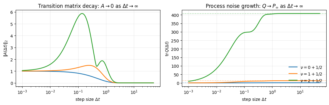

Dotted horizontal lines mark $\mathrm{tr}\,P_\infty$ for each order — the asymptote $Q$ relaxes onto. Higher-order Materns relax slower (more oscillatory state coordinates carry inertia), but the limit is the same.

4. Sample paths via forward simulation of the discrete-time SDE¶

We can draw GP sample paths without ever forming a dense Gram matrix. The recipe is the standard linear-Gaussian forward simulation of the discrete state-space model:

Sample $\mathbf{x}_0 \sim \mathcal{N}(0, P_\infty)$ .
For $k = 0, 1, \dots, N-1$ : sample $\mathbf{x}_{k+1} = A_k \mathbf{x}_k + \mathbf{q}_k$ with $\mathbf{q}_k \sim \mathcal{N}(0, Q_k)$ .
Read out $f_k = H\,\mathbf{x}_k$ .

All work is local in time; no $N \times N$ Cholesky. We compare paths drawn this way against paths drawn from the dense Matern Cholesky for the same time grid.

def sample_sde_paths(
    sde: MaternSDE,
    times: jnp.ndarray,
    n_paths: int,
    key: jax.Array,
) -> jnp.ndarray:
    """Forward-simulate ``n_paths`` realisations of the discrete state-space model."""
    _F, _L, H, _Q_c, P_inf = sde.sde_params()
    d = sde.state_dim
    dts = jnp.diff(times)
    A_all, Q_all = sde.discretise(dts)
    L_inf = jnp.linalg.cholesky(P_inf + 1e-10 * jnp.eye(d))
    L_step = jnp.linalg.cholesky(Q_all + 1e-10 * jnp.eye(d)[None])

    key_init, key_step = jr.split(key)
    x0 = L_inf @ jr.normal(key_init, (d, n_paths))  # (d, n_paths)
    eps = jr.normal(key_step, (dts.shape[0], d, n_paths))

    def step(
        x_prev: jnp.ndarray, inputs: tuple[jnp.ndarray, jnp.ndarray, jnp.ndarray]
    ) -> tuple[jnp.ndarray, jnp.ndarray]:
        A_k, L_k, eps_k = inputs
        x_next = A_k @ x_prev + L_k @ eps_k
        return x_next, x_next

    _, xs = jax.lax.scan(step, x0, (A_all, L_step, eps))
    states = jnp.concatenate([x0[None], xs], axis=0)  # (N, d, n_paths)
    f_paths = jnp.einsum("ij,njp->np", H, states)  # (N, n_paths)
    return f_paths


def sample_dense_paths(
    sde: MaternSDE,
    times: jnp.ndarray,
    n_paths: int,
    key: jax.Array,
) -> jnp.ndarray:
    X = times[:, None]
    K = matern_kernel(X, X, sde.variance, sde.lengthscale, nu=float(sde.nu))
    K = K + 1e-8 * jnp.eye(X.shape[0])
    L = jnp.linalg.cholesky(K)
    return L @ jr.normal(key, (X.shape[0], n_paths))


N = 320
times = jnp.linspace(0.0, 4.0, N)
n_paths = 4
seed = 0

fig, axes = plt.subplots(3, 2, figsize=(12, 7.5), sharex=True)
for row, (_p, sde) in enumerate(sdes.items()):
    sde_paths = sample_sde_paths(sde, times, n_paths, jr.PRNGKey(seed))
    dense_paths = sample_dense_paths(sde, times, n_paths, jr.PRNGKey(seed + 1))
    for j in range(n_paths):
        axes[row, 0].plot(times, sde_paths[:, j], lw=1.2, alpha=0.85)
        axes[row, 1].plot(times, dense_paths[:, j], lw=1.2, alpha=0.85)
    axes[row, 0].set_ylabel(rf"Matern-{int(2 * sde.nu)}/2")
    for ax in axes[row]:
        ax.grid(alpha=0.2)
        ax.axhline(0.0, color="k", lw=0.4, alpha=0.4)
axes[0, 0].set_title("SDE forward-simulation paths")
axes[0, 1].set_title("Dense Matern Cholesky paths")
for ax in axes[-1]:
    ax.set_xlabel("t")
fig.suptitle("Same statistics, different generation path")
fig.tight_layout()
plt.show()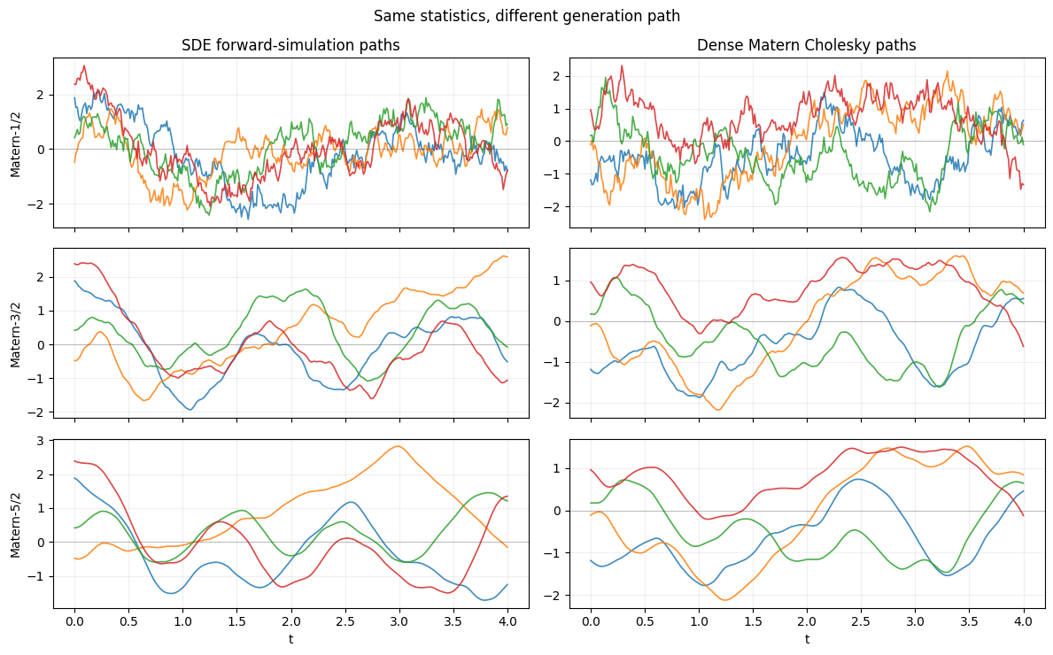

Each row pairs the same kernel order; the seeds differ across columns so the realisations are independent draws. Visually the rougher Matern-1/2 paths sit on top, the smoother Matern-5/2 paths at the bottom, with the SDE and dense columns indistinguishable in their statistical character. The variances and correlation lengths match by construction.

5. Empirical covariance of SDE samples matches the analytic kernel¶

A stronger check than visual matching: estimate the covariance $\hat C_{ij} = \mathrm{Cov}[f(t_i), f(t_j)]$ from many SDE-simulated paths and compare to the closed-form Matern Gram on the same grid.

n_mc = 2000
mc_times = jnp.linspace(0.0, 2.0, 41)

fig, axes = plt.subplots(1, 3, figsize=(13.5, 4.0))
for ax, (p, sde) in zip(axes, sdes.items(), strict=False):
    paths = sample_sde_paths(sde, mc_times, n_mc, jr.PRNGKey(11 + p))  # (N, n_mc)
    paths_centered = paths - paths.mean(axis=1, keepdims=True)
    C_emp = (paths_centered @ paths_centered.T) / (n_mc - 1)
    K_true = matern_kernel(
        mc_times[:, None],
        mc_times[:, None],
        sde.variance,
        sde.lengthscale,
        nu=float(sde.nu),
    )
    ax.plot(
        mc_times, jnp.diag(C_emp), label=r"$\widehat{\mathrm{Var}}\,f(t)$ (MC)", lw=1.7
    )
    ax.plot(mc_times, jnp.diag(K_true), "--", label=r"$\sigma^2$", lw=1.4)
    ax.plot(
        mc_times,
        C_emp[:, 0],
        lw=1.7,
        label=r"$\widehat{\mathrm{Cov}}\,(f(0), f(t))$ (MC)",
    )
    ax.plot(mc_times, K_true[:, 0], "--", lw=1.4, label=r"$k(t, 0)$")
    ax.set_title(rf"Matern-{int(2 * sde.nu)}/2  ({n_mc} paths)")
    ax.set_xlabel("t")
    ax.grid(alpha=0.25)
axes[0].legend(frameon=False, loc="upper right", fontsize=8)
fig.suptitle(
    "Empirical covariance from SDE samples agrees with the analytic Matern kernel"
)
fig.tight_layout()
plt.show()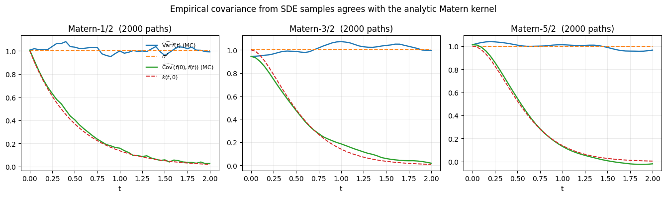

Solid lines are Monte-Carlo estimates from $n_\text{mc} = 2000$ forward simulations; dashed lines are the closed-form values. They overlap to the precision afforded by 2000 samples.

6. The kernel zoo — primitives and composition rules¶

Matern alone is enough to cover smooth time series, but real signals usually have more structure: a fixed offset, a carrier oscillation, an annual cycle, a quasi-periodic modulation. State-space form scales gracefully here too — every additional kernel is another small block in the state, not another factor of $N$ in inference cost.

This section walks through the four new primitive / composition kernels added on top of MaternSDE:

Class	Math	State dim
`ConstantSDE(σ²)`	$k(\tau) = \sigma^2$	1
`CosineSDE(σ², ω)`	$k(\tau) = \sigma^2 \cos(\omega\,\tau)$	2
`PeriodicSDE(σ², ℓ, T, J)`	MacKay periodic, Fourier-truncated to $J$ harmonics	$1 + 2J$
`SumSDE((k₁, …))`	$k(\tau) = \sum_i k_i(\tau)$	$\sum_i d_i$
`ProductSDE(k₁, k₂)`	$k(\tau) = k_1(\tau)\,k_2(\tau)$	$d_1 \cdot d_2$
`QuasiPeriodicSDE(matern, periodic)`	thin wrapper for `ProductSDE`	$d_M (1 + 2J)$

SumSDE is block-diagonal in $F$ , $L$ , $Q_c$ and $P_\infty$ , with the readouts $H$ concatenated. ProductSDE uses Kronecker-sum drift $F = F_1 \otimes I + I \otimes F_2$ and Kronecker-product readout / stationary covariance $H = H_1 \otimes H_2$ , $P_\infty = P_{\infty,1} \otimes P_{\infty,2}$ . The diffusion is a sum of two Kronecker terms — see the ProductSDE docstring for the full formula.

from pyrox.gp import (
    ConstantSDE,
    CosineSDE,
    PeriodicSDE,
    ProductSDE,
    QuasiPeriodicSDE,
    SumSDE,
)
from pyrox.gp._src.kernels import periodic_kernel

6.1 Building blocks: ConstantSDE, CosineSDE, PeriodicSDE¶

We instantiate one of each, draw a few sample paths via the same forward-simulation recipe used for Matern in §4, and overlay the SDE autocovariance against a dense reference where one is available. PeriodicSDE uses n_harmonics = 7 — enough to match the MacKay periodic kernel to better than 1e-4 in the typical hyperparameter regime.

const = ConstantSDE(variance=0.6)
cos = CosineSDE(variance=1.0, frequency=2.0 * jnp.pi)  # period 1
per = PeriodicSDE(variance=1.0, lengthscale=1.0, period=1.0, n_harmonics=7)

primitives = {"ConstantSDE": const, "CosineSDE": cos, "PeriodicSDE": per}

times_demo = jnp.linspace(0.0, 4.0, 320)
fig, axes = plt.subplots(3, 2, figsize=(13, 7.8), sharex="col")
for row, (name, sde) in enumerate(primitives.items()):
    paths = sample_sde_paths(sde, times_demo, n_paths=4, key=jr.PRNGKey(7 + row))
    for j in range(4):
        axes[row, 0].plot(times_demo, paths[:, j], lw=1.1, alpha=0.85)
    axes[row, 0].set_ylabel(name)
    axes[row, 0].grid(alpha=0.25)
    axes[row, 0].axhline(0.0, color="k", lw=0.4, alpha=0.4)

    F, _L, H, _Q_c, P_inf = sde.sde_params()
    taus_demo = jnp.linspace(0.0, 4.0, 401)
    K_sde = jax.vmap(
        lambda t, F=F, H=H, P_inf=P_inf: (H @ jsl.expm(F * t) @ P_inf @ H.T).squeeze()
    )(taus_demo)
    axes[row, 1].plot(taus_demo, K_sde, lw=1.8, label="SDE autocov", color="C0")
    if name == "ConstantSDE":
        axes[row, 1].axhline(0.6, ls="--", lw=1.3, color="C3", label=r"$\sigma^2$")
    elif name == "CosineSDE":
        axes[row, 1].plot(
            taus_demo,
            jnp.cos(2.0 * jnp.pi * taus_demo),
            "--",
            lw=1.3,
            label=r"$\sigma^2 \cos(\omega\tau)$",
        )
    else:
        K_dense = periodic_kernel(
            taus_demo[:, None],
            jnp.zeros((1, 1)),
            jnp.asarray(1.0),
            jnp.asarray(1.0),
            jnp.asarray(1.0),
        ).squeeze()
        axes[row, 1].plot(taus_demo, K_dense, "--", lw=1.3, label="MacKay periodic")
    axes[row, 1].grid(alpha=0.25)
    axes[row, 1].legend(frameon=False, loc="upper right", fontsize=8)
axes[0, 0].set_title("Sample paths")
axes[0, 1].set_title("Autocovariance vs reference")
for ax in axes[-1]:
    ax.set_xlabel("t" if ax is axes[-1, 0] else r"lag $\tau$")
fig.suptitle("Primitive SDE kernels: paths and autocovariance")
fig.tight_layout()
plt.show()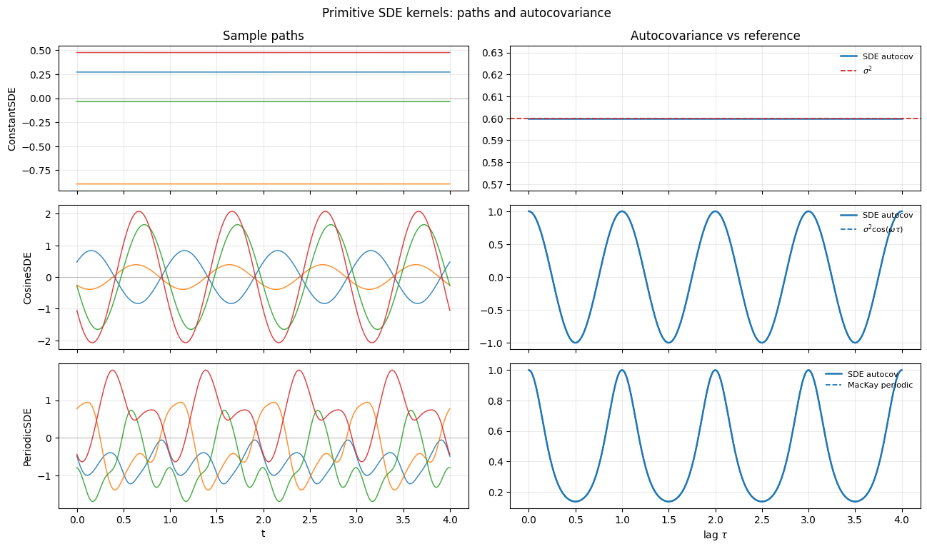

ConstantSDE paths are flat realisations: each draw is a single Gaussian random variable replicated across time. The autocovariance is the constant $\sigma^2$ .
CosineSDE paths are pure sinusoids with random amplitude and phase. The covariance oscillates exactly as $\sigma^2 \cos(\omega\tau)$ .
PeriodicSDE paths are smooth, period-aware, and not sinusoidal — they live in the function space of the MacKay periodic kernel. Truncating the Fourier expansion at $J=7$ matches the dense kernel within plotting precision.

6.2 Composition: trend + offset via `SumSDE`¶

A common modelling pattern is “smooth trend on top of a fixed offset”. With dense kernels this is one line: RBF + Constant. In state-space form it’s exactly the same — just SumSDE. The block-diagonal construction keeps each component’s state space disjoint, so the cost is purely additive ( $\sum_i d_i$ ).

trend = SumSDE(
    (
        MaternSDE(variance=0.7, lengthscale=0.8, order=1),
        ConstantSDE(variance=0.4),
    )
)
print(f"SumSDE state dim: {trend.state_dim}  (= 2 + 1)")

paths = sample_sde_paths(trend, times_demo, n_paths=6, key=jr.PRNGKey(33))

fig, axes = plt.subplots(1, 2, figsize=(12, 3.6))
for j in range(6):
    axes[0].plot(times_demo, paths[:, j], lw=1.1, alpha=0.85)
axes[0].set_title("MaternSDE-3/2 + ConstantSDE — sample paths")
axes[0].set_xlabel("t")
axes[0].grid(alpha=0.25)

F, _L, H, _Q_c, P_inf = trend.sde_params()
taus_demo = jnp.linspace(0.0, 3.0, 301)
K_sum = jax.vmap(lambda t: (H @ jsl.expm(F * t) @ P_inf @ H.T).squeeze())(taus_demo)
K_truth = (
    matern_kernel(
        taus_demo[:, None],
        jnp.zeros((1, 1)),
        jnp.asarray(0.7),
        jnp.asarray(0.8),
        nu=1.5,
    ).squeeze()
    + 0.4
)
axes[1].plot(taus_demo, K_sum, lw=2.2, label=r"$H \exp(F\tau) P_\infty H^\top$")
axes[1].plot(taus_demo, K_truth, "--", lw=1.3, label=r"$k_M(\tau) + \sigma_C^2$")
axes[1].set_title("Autocovariance: SumSDE matches dense sum")
axes[1].set_xlabel(r"lag $\tau$")
axes[1].grid(alpha=0.25)
axes[1].legend(frameon=False, loc="upper right")
fig.tight_layout()
plt.show()

SumSDE state dim: 3  (= 2 + 1)

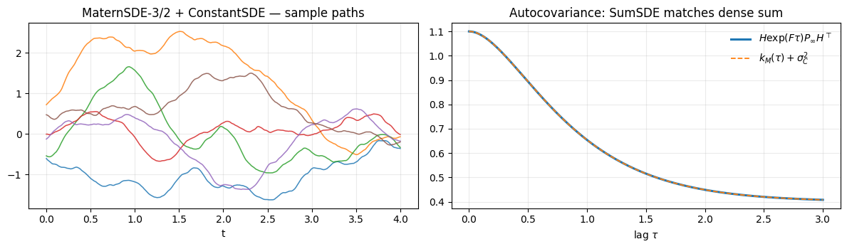
Sample paths show the Matern wiggle riding on independently-drawn constant offsets — exactly the prior we wanted. The autocovariance recovers $k_{\rm Matern}(\tau) + \sigma_C^2$ to machine precision.

6.3 Composition: damped oscillation via `ProductSDE`¶

The product of a Matern and a Cosine is the subband Matern kernel — a stationary kernel whose spectral density is centred on a non-zero carrier $\omega_0$ . It’s the right prior for narrowband oscillatory signals (audio harmonics, geophysical resonances, modulated sensor traces). State dim is $d_M \cdot d_C$ — for Matern-3/2 × Cosine that’s $2 \cdot 2 = 4$ .

damped = ProductSDE(
    MaternSDE(variance=1.0, lengthscale=0.6, order=1),
    CosineSDE(variance=1.0, frequency=2.0 * jnp.pi * 1.5),  # 1.5 Hz carrier
)
print(f"ProductSDE state dim: {damped.state_dim}")

paths = sample_sde_paths(damped, times_demo, n_paths=4, key=jr.PRNGKey(101))

fig, axes = plt.subplots(1, 2, figsize=(12, 3.6))
for j in range(4):
    axes[0].plot(times_demo, paths[:, j], lw=1.1, alpha=0.85)
axes[0].set_title("MaternSDE-3/2 x CosineSDE — sample paths")
axes[0].set_xlabel("t")
axes[0].grid(alpha=0.25)

F, _L, H, _Q_c, P_inf = damped.sde_params()
taus_demo = jnp.linspace(0.0, 2.0, 401)
K_prod = jax.vmap(lambda t: (H @ jsl.expm(F * t) @ P_inf @ H.T).squeeze())(taus_demo)
K_m = matern_kernel(
    taus_demo[:, None], jnp.zeros((1, 1)), jnp.asarray(1.0), jnp.asarray(0.6), nu=1.5
).squeeze()
K_c = jnp.cos(2.0 * jnp.pi * 1.5 * taus_demo)
axes[1].plot(taus_demo, K_prod, lw=2.2, label=r"ProductSDE autocov")
axes[1].plot(
    taus_demo,
    K_m * K_c,
    "--",
    lw=1.3,
    label=r"$k_{\rm Matern}(\tau)\,\cos(\omega_0\tau)$",
)
axes[1].set_title("Autocovariance: ProductSDE matches dense product")
axes[1].set_xlabel(r"lag $\tau$")
axes[1].grid(alpha=0.25)
axes[1].legend(frameon=False, loc="upper right")
fig.tight_layout()
plt.show()

ProductSDE state dim: 4

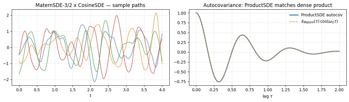
The paths are oscillations whose envelope drifts on the Matern lengthscale — a damped carrier signal. The product autocovariance matches $k_M(\tau) \cos(\omega_0 \tau)$ to numerical precision (the slight curvature of the envelope reflects the Matern factor).

6.4 Quasi-periodic kernels — modulated periodic structure¶

The classic “stellar” prior: a periodic signal whose amplitude drifts slowly over time. Mathematically it’s $k_{\rm Matern}(\tau) \cdot k_{\rm Periodic}(\tau)$ — a ProductSDE of two stationary kernels. QuasiPeriodicSDE is just a thin convenience wrapper that documents the standard recipe.

qp = QuasiPeriodicSDE(
    MaternSDE(variance=1.0, lengthscale=2.5, order=1),  # slow envelope (long ell)
    PeriodicSDE(variance=1.0, lengthscale=1.0, period=0.6, n_harmonics=5),
)
print(f"QuasiPeriodicSDE state dim: {qp.state_dim}  (= 2 * (1 + 2*5))")

paths = sample_sde_paths(qp, times_demo, n_paths=4, key=jr.PRNGKey(57))

fig, ax = plt.subplots(1, 1, figsize=(13, 3.4))
for j in range(4):
    ax.plot(times_demo, paths[:, j], lw=1.1, alpha=0.85)
ax.set_title(
    "QuasiPeriodicSDE: Matern-3/2 (ell=2.5) x Periodic (period=0.6, J=5) — modulated cycles"
)
ax.set_xlabel("t")
ax.axhline(0.0, color="k", lw=0.4, alpha=0.4)
ax.grid(alpha=0.25)
fig.tight_layout()
plt.show()

QuasiPeriodicSDE state dim: 22  (= 2 * (1 + 2*5))

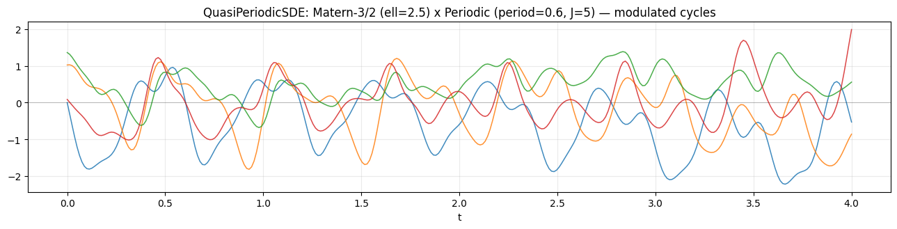
Each draw shows a clear period of about 0.6 time units, but the amplitude drifts on a slow Matern timescale — short bursts of high-amplitude oscillation followed by quiescent stretches, exactly the prior class used for stellar light curves and modulated seasonal signals.

What this PR ships and what comes next¶

PR 1 (issue #37 partial, #112 — already merged). The SDEKernel protocol and the MaternSDE family for $\nu \in \{1/2, 3/2, 5/2\}$ .

This PR (issue #37 finish). The kernel zoo on top of MaternSDE:

Primitives: ConstantSDE, CosineSDE (closed-form rotation discretise), PeriodicSDE (Solin & Sarkka 2014, Fourier-truncated MacKay periodic kernel via a stable log-space Bessel helper).
Composition rules: SumSDE (block-diagonal) and ProductSDE (Kronecker-sum drift, Kronecker-product readout / stationary covariance, with the diffusion matrix derived from the Lyapunov identity).
Convenience: QuasiPeriodicSDE as a documented ProductSDE(MaternSDE, PeriodicSDE).

Next up — issue #38. MarkovGPPrior plus the Kalman filter / RTS smoother. Once that lands, every kernel above can be plugged directly into a NumPyro model with linear-time temporal inference: f = numpyro.sample("f", MarkovGPPrior(QuasiPeriodicSDE(...), times)).

References.

Sarkka, S. & Solin, A. (2019). Applied Stochastic Differential Equations. Cambridge University Press, Ch. 12.
Hartikainen, J. & Sarkka, S. (2010). Kalman Filtering and Smoothing Solutions to Temporal Gaussian Process Regression Models. IEEE MLSP.
Solin, A. & Sarkka, S. (2014). Explicit Link Between Periodic Covariance Functions and State Space Models. AISTATS.
Wilkinson, W. J., Sarkka, S. & Solin, A. (2023). Bayes-Newton Methods for Approximate Bayesian Inference with PSD Guarantees. JMLR 24(83).